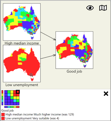
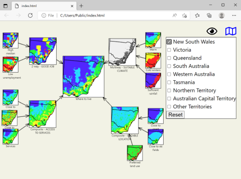
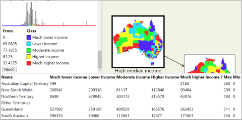
This publication (and any material sourced from it) should be attributed as MCAS-S Development Partnership 2022, Multi-Criteria Analysis Shell for Spatial Decision Support MCAS-S version 4 User guide, ABARES, Canberra, March. CC BY-ND 4.0 https://doi.org/10.25814/kafw-xy28

1 Getting started

MCAS-S runs on most standard computers. To get started with MCAS-S you will need:

1. Software: Install the MCAS-S software onto your computer (see 1.2 Installation)
2. Data: 

• Download, unzip and open the Where to live sample project [zip 190 MB] or other data from the MCAS-S website or 
• load and open your own MCAS-S project and data (see section 5.5 Preparing your own data). 
• The MCAS-S sample project and the selection of Australian national map layers available from the website are used as examples throughout this user guide.
• The MCAS-S Quick Start Guide also provides a short introduction to the basics of performing multi-criteria analysis with MCAS-S by analysing the possible spread of an aquatic invasive species across Australia.

1.1 System Requirements

MCAS-S installation requirements

• 64-bit operating system (if you require older 32-bit software please contact the MCAS-S team)
• Windows 10 or later
• 8 GB of RAM (minimum recommended)
• 500MB disk space for program 
• 1GB disk space for data layers.

1.2 Installation

To install the MCAS-S desktop application onto your PC (note MCAS-S does not run on a Mac but can run on a virtual PC):

1. Download the latest version 4 MCAS-S installer from the MCAS-S website. 
2. Save the MCAS-S installer on your computer in case the program needs to be repaired later. 
3. Uninstall any old versions of MCAS-S version 4 (It is still possible to run older versions of MCAS-S such as 3.2 on the same computer for old projects).
4. Double-click the MCAS-S installer and follow the installation instructions. Install the software on a local hard drive. The default location is C:\Program Files\ABARES\Multi-Criteria Analysis Shell v4.
5. The MCAS-S icon (Figure 1) is added to the desktop when successfully installed.
6. Double-click the MCAS-S icon to open the software. The screen shown at Figure 2 will appear. The text at the left-hand side of the screen provides links to the MCAS-S user guide, the MCAS-S website and information on the development partners. 

Figure 1 MCAS-S desktop icon

Figure 2 MCAS-S interface

Install an MCAS-S project and data

To use MCAS-S you will also need to install, and open, a new or existing MCAS-S project and map layers using one of the following options:

• Option 1)    Download the sample project (or other data such as Australian National Map layers) from the MCAS-S website. Check that there is enough available space on your drive as the entire set of 1km Australian National Map layers require 4GB. Download or copy and save the Data folder and project to the working directory. The data and project need to be saved in the same folder.
• Option 2)    Download or locate an existing project and data structure from another source.
• Option 3)    Follow steps to set up your own project and data structure at section 5.5 Preparing your own data.

IMPORTANT: MCAS-S projects MUST be saved alongside the project data. This location can be any working drive or directory and does not need to be where the software is saved.

1.3 Opening a project

There are two options to open an existing project: 

• Option 1)    Navigate to and select the project filename using Microsoft Windows Explorer or similar. Double click to open the project.
• Option 2)    Open MCAS-S using the desktop icon. MCAS-S will start and the screen shown in Figure 2 will appear. Go to the File drop-down menu, select Open, and navigate to the project. 

Where is the sample project?

You will find the sample project on the MCAS-S website. Choose either the ‘blank’ sample project to start with an empty project window or the ‘Where to live’ sample to see the data layers combined to show a hypothetical example of where to live in Australia. 

Using a project created in an earlier version of MCAS-S

If you open a project from an earlier version of MCAS-S the classifications may be lost. Compare the old project with the new version and reclassify layers where necessary. You may also need to reselect masks and overlays. 

1.4 Creating a new project

To create a new project use the File drop-down menu and select New. Then choose between three options (Figure 3):

• Option 1)    Store alongside open project, reusing project data—this creates a copy of your open project and is like the Save as option. 
• Option 2)    Create alongside existing project, reusing project data—this creates a new black project associated with an existing Data folder. Type in the name of the new project then browse to and save alongside the required Data folder.
• Option 3)    Create new project folder structure—this will create a new project and a new empty Data folder structure in the directory that you specify. Use this option if using your own project data layers. Fill the new empty Data folders with your project data as described in section 5.5 Preparing your own data so you can begin work. You can use your own pre-processed data or a subset of an existing, larger dataset, by copying and pasting from an existing dataset to the Primary data, Overlay data and Mask data project files of the new project. (Note that GIS software may be needed to copy individual grids to avoid corruption so it is safer to copy over entire folders.)

Once the new project is open, the primary data grids, overlays and masks saved in the Data folder will be available to use.

Figure 3 Options for creating a new project

1.5 Saving an open project

To save an open project use the File drop-down menu and select Save. This will also save a copy in the History folder see section 8.3.5 Restoring a previous version of the MCAS-S workspace from the History folder. 

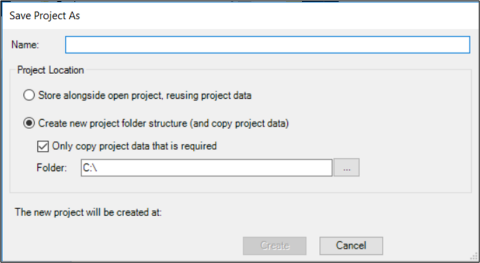
To save a copy of an open project select Save as. The Save Project As window then provides two options (Figure 4):

Option 1)    Store alongside open project, reusing project data—allows you to keep working in the same place with an exact duplicate of your existing project

Option 2)    Create new project folder structure (and copy project data) —creates an entirely new copy of the project and data which can be saved in a new location. You can choose to copy the entire data folder, or just the data layers in use.

• a.    To copy all data: Do not check the box Only copy project data that is required (default). If the check box is not selected, then the entire data folder will be copied to the new project regardless of which data layers are used in the project at the time. The data folder may be very large so make sure that there is enough space in the new location before selecting this option. 
• b.    To copy only data in use: If the new project only needs some of the data layers from the data folder choose Only copy project data that is required. Selecting this check box means that the data folder for the new project will ONLY contain data layers which show in the project window of the open MCAS-S project. The new data folder will include primary or classified data layers which have been dragged into the workspace, and selected overlays and masks which are in use. 

Figure 4 Save as project window copying only required datasets

1.6 Introduction to the display workspace: available features and functions

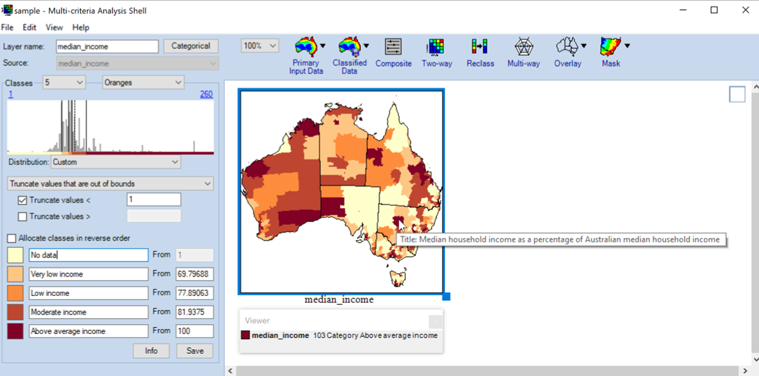
You can use MCAS-S functions to allow users to interact with spatial data at every stage of your project. Figure 5, Figure 6, and Figure 7 show the MCAS-S display workspace and where to find key functions once a project is open.
MCAS-S selects analysis functions and interface panels according to map type. The display and analysis functions change automatically when you access different types of spatial display maps, such as raw input data, composite indicators, and two-way and multi-way comparisons of datasets. Figure 7 shows the MCAS-S workspace configured for a continuous primary data layer. Section 5.1 Primary input data explains the difference between categorical and continuous data. These features make the MCAS-S interface very intuitive to use.

Figure 5 MCAS-S interface

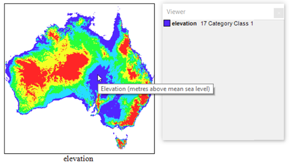
Hover the mouse over the top panel to see a tool tip with more information (Figure 6). 

Figure 6 Tool tip describing the Primary Input Data

Figure 7 MCAS-S functions in the left-hand side interface panel

Note: The figure shows locations of MCAS-S functions once you have added and selected a continuous primary data layer. The left-hand interface panel display will change if the Categorical button is selected. The right-hand side is referred to as the workspace.

2    Introduction

Why use MCAS-S?

MCAS-S is a tool to view and combine mapped information. MCAS-S can inform spatial decision making and help with stakeholder engagement and communication. MCAS-S is powerful and easy to use.
MCAS-S projects are:

• transparent – you can see all the inputs used to meet an objective and how these are combined 
• flexible – you can use MCAS-S to compare options and explore trade-offs. You can use your own input data  
• fast – immediately see changes to your objective when any input or combination method changes. 

Who creates MCAS-S?

The Multi-Criteria Analysis Shell for Spatial Decision Support (MCAS-S) software was created by the Australian Bureau of Agricultural and Resource Economics and Sciences (ABARES) with the support of the MCAS-S Development Partnership. The MCAS-S Development Partners was formed in 2013 to promote the use and improvement of the MCAS-S software. 

What data does MCAS-S use?

The sample project includes a limited selection of Australian national map layers which are ready for use. This and other data are available from the MCAS-S website. You can also format your own data to use in MCAS-S projects. 

2.1 Who can use this decision support tool?

MCAS-S is designed for decision-makers. It shows transparently how mapped information can be combined to meet an objective. MCAS-S allows stakeholders to see the effects that their decisions may have.
MCAS-S makes it easier to analyse spatial information without Geographic Information Systems (GIS) programming, 
What does MCAS-S do?
MCAS-S is a map viewer and an easy-to-use spatial-analysis tool. MCAS-S helps you to:

• view and classify map layers
• compare and combine map layers
• clearly show the relationship between data layers and objectives
• look at alternative views quickly using interactive ‘live-update’ mapping options
• produce fast statistical reports by region
• document your assumption, decision process and results.

What do I need to consider?

MCAS-S helps you to answer ‘where questions’ when you have access to appropriate spatial input data, expert knowledge, an understanding of thresholds and linkages between the data. 

Since MCAS-S will allow you to carry out potentially inappropriate and invalid data associations, you should take advantage of expert opinion and stakeholder advice, and clearly articulate your results including the data dependencies and assumptions.

Where does Multi-Criteria Analysis fit in?

MCAS-S software can facilitate spatial multi-criteria analysis (MCA)—a process designed to improve decision-making by involving diverse factual information, value judgement, opinion, and policy and management goals. MCAS-S is particularly useful for demonstrating a logical and transparent framework for spatial information. MCA is discussed in more detail in section 3 Multi-criteria analysis.

2.2 What’s new in version 4

This new version of the MCAS-S software (version 4) includes the following new features:

• Better performance
  • faster display of list of available primary data layers using a cached display, 
  • out of memory error corrected. 
• Easier to view and share
  • More zoom and pan options
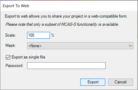
  • Share simple projects with non-MCAS-S users to view in their web browser 
• Easier to organise your data and projects
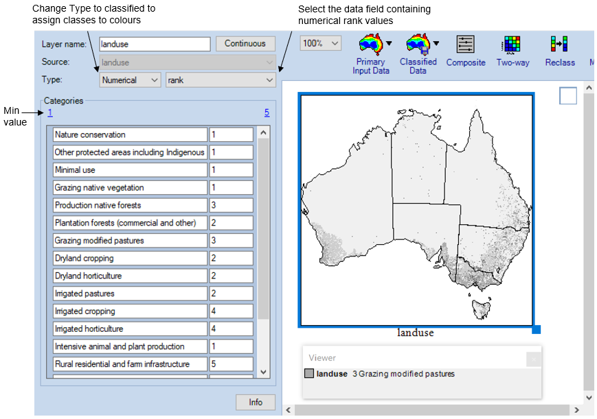
  • sort categorical data classes alphabetically, use class names and numerical categorical rank values directly from data fields,
  • see the data layer source file name to make it easier to fix broken links even if you’ve changed the display name in MCAS-S,
  • mask using primary data layers (no need to duplicate layers in the primary and mask folders therefore reducing the size of your data packs), 
  • save linked projects (find and view the MCAS-S project used to create classified layers while you are using them).

Detailed instructions on all functions are included in this user guide. We hope you enjoy using the new version. 

3    Multi-criteria analysis

Multi-criteria analysis (MCA) is one approach to assess complex issues in coupled human–environment systems. It is widely applied in business, government and community decision-making, particularly in natural resource management. Spatial MCA is a process to assist decision-makers—it does not do the decision-making, but it can be used to explore options and potential outcomes. 
Well-developed MCA approaches: 

• are highly flexible and relatively simple to use
• enable the capture of quantitative and qualitative data and issues
• permit the development of scenarios
• allow trade-offs to be explored
• enable the stakeholder to factor MCA results into the decision-making processes.

There are five steps in the MCA assessment process (Figure 8). Each stage of the MCA process should be carried out rigorously, in parallel with stakeholder engagement.

Figure 8 Multi-criteria analysis process

This guide shows how MCAS-S can be used to follow the steps in an MCA. Note that the MCAS-S tool is not restricted to use in MCA assessments. It can be used in any situation where there is the need to display, combine and investigate the relationships between spatial information. 

Will MCAS-S be useful for my project?

Spatial MCA using MCAS-S is likely to be useful when:

• The question involves a location component; such as ‘Where to live in Australia?’
• You want to combine diverse information such as environmental, social and economic, value judgements, stakeholder viewpoints, and or policy and management goals.
• It will be important to justify your conclusions based on informed, systematic and transparent analysis.
• You would like the flexibility to explore: how achievable an outcome might be, possible compromise scenarios, or sensitivity to data quality or uncertainty.  

Throughout this manual a hypothetical example—‘Where to live in Australia’ shows how the MCAS-S software can be used in a multi-criteria analysis. Follow the development of the ‘Where to live in Australia’ project in the boxed text in each section. The example starts by identifying issues to consider (Box 1) and results in a completed MCAS-S project (Box 2). To begin see section 4 Step 1: Define the objective and decision criteria.

4    Step 1: Define the objective and decision criteria

The first step, ‘Define the objective and decision criteria’, is critical to success in an MCA process, as this frames the assessment and determines the subsequent steps in the process. 
It is recommended that you consult a range of experts and stakeholders to develop a ‘means-to-an-end’ diagram to represent the objective and decision criteria, and to decide what data will be required and how they might be combined.

Means-to-an-end diagrams

Figure 9 shows an example of a simple means-to-an-end diagram, which is explained in more detail in Box 1, and shown as a completed MCAS-S project in Box 2.

Box 1    Where to live—issues to consider

The example of ‘Where to live’ shows how the MCAS-S software can be used in a multi-criteria analysis. 

In this example the objective is to identify places to live in Australia based on employment, suitable climate, access to services and lifestyle. 
Figure 9 shows a simple example means-to-an-end diagram. This example uses input data from the sample project, however the way in which this data has been combined to identify ‘Where to live’ is hypothetical and is included to show how an MCA could be structured. Other factors and input data could be included, such as land price, cost of living, extreme weather events and natural disasters, locations of hospitals and schools etc. In this case the stakeholders might be a family. However other examples are likely to require consultation with relevant experts to define the objective and decision criteria. Published example projects are on the MCAS-S website.

Figure 9 A means-to-an-end diagram

MCAS-S lets you build a view that satisfies your stated objective by combining primary data layers into criteria or composites. 
A means-to-an-end diagram provides a structure to follow in creating your MCAS-S project. This process will also help to match the spatial and temporal scale of the input information and analysis to the objective, which is a critical consideration.

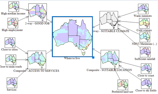
Box 2    Where to live—means-to-an-end diagram in MCAS-S

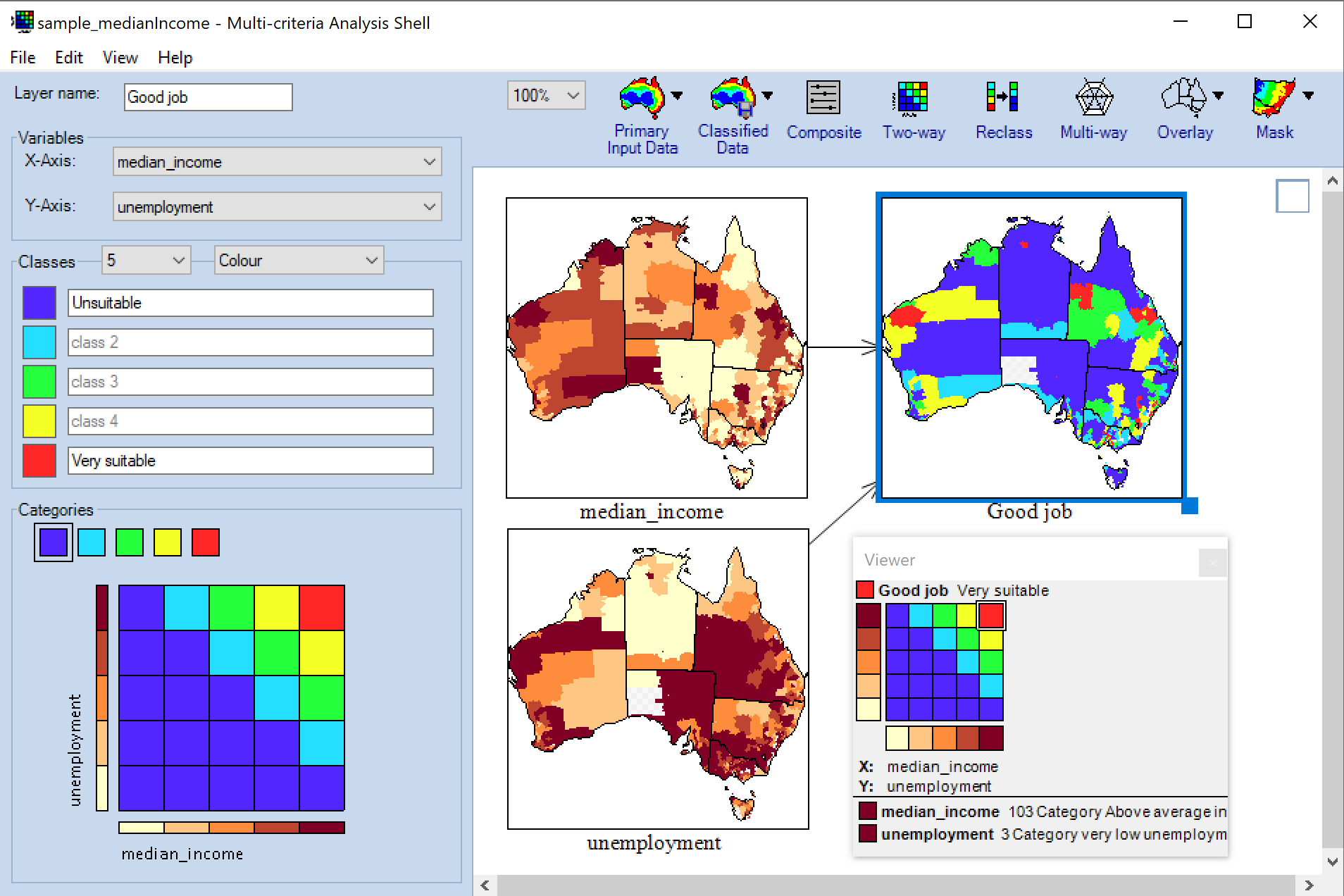
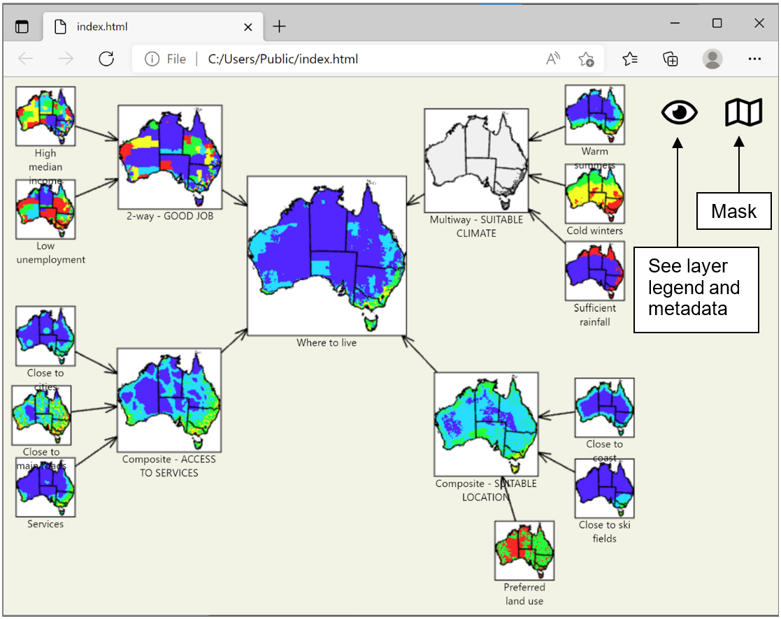
A means-to-an-end diagram, like the one in Figure 9, can be represented by data layers in MCAS-S.
The ‘Where to live’ layer, is shown on the right-hand side of the figure below, with the input criteria and primary data layers shown on the left.

5    Step 2: Assemble data inputs

Once you have installed MCAS-S and opened a blank or existing project, you can add data to the display workspace. 

TIP: To bring in a new layer—click and drag

Types of data

MCAS-S allows you to work with four types of data:

• primary input data—gridded raster input layers for display and for undertaking analysis (section 5.1 Primary input data)
• classified data—gridded raster data layers that you create and export using MCAS-S (section 5.4 Classified data—if you have just begun using MCAS-S there may not be any layers in the classified folder)
• overlay data—contextual vector data, lines or points for visual reference (such as rivers or towns see section 5.2 Overlay data)
• mask data—gridded raster layers used to restrict the area of analysis or define regions for reporting (section 5.3 Mask data).

Steps to add data layers, masks or overlays

1. Select the Primary, Classified, Overlay or Mask menu to expand and view the available layers 
2. Click and drag to bring in primary, classified, or overlay layers into the workspace. Multiple layers can be added to the workspace by holding down the shift key when selecting layers and then dragging in all the selected layers.
3. Check the box next to an overlay or mask of interest to apply the selection to all layers open in the project 

Where can I find data for MCAS-S?

You can download ready to use data packs for Australia from the MCAS-S website. These include primary, overlay and mask data layers. However, your project may require other data inputs, which you can prepare for use in MCAS-S using a GIS. Ensure that any data packs which are downloaded or created conform to the folder structure shown in section 5.5 Preparing your own data.  

5.1 Primary input data

What are primary input data?

The Primary folder contains data layers for display and analysis. Primary data are gridded or raster data.
Steps to add primary input data to a project

1. Select primary input data layers from a drop-down menu (under the heading Primary Input Data). Data layers can be sorted into separate folders under the Primary folder. The left hand side of the drop down menu shows these folders. 
2. Bring layers into the display workspace by clicking and dragging them in from the right hand side of the menu with the mouse (Figure 10).

Figure 10 Primary data icons for categorical and continuous primary input data

The three different icons in the Primary data folder indicate categorical, continuous and time series as shown in Figure 10. To see what your data might look like as continuous or categorical see Figure 11. You can switch between these views using the button on the interface panel.

Figure 11 Compare categorical and continuous primary input data display

Note: The data layer ‘ra’ remoteness has been dragged from the Primary Input Data menu into the display workspace. The figure shows the default display and interface panel for categorical (all classes blue) and continuous (5 classes coloured by value). 

5.1.1    Categorical data

What are categorical data?

Categorical data are a type of primary data for use in MCAS-S analysis. Categorical data are grouped or categorised according to some common property, such as soil type or vegetation type. The data have labels that describe a category or group of interest. The categorical data icon indicates that MCAS-S recognises the labels for the data classes from a (.txt) file with the same name as the data layer, or from a field in the data attribute table. The text file is saved in the same data layer folder, or the label field has been specified in the .tip file (see section 6.2.2 Classifying categorical data). 

How will categorical data display in MCAS-S?

When a categorical dataset is dragged into the workspace all categories from the text file are initially assigned to the lowest class (dark blue). Figure 11 shows how a layer will look when dragged into the MCAS-S workspace from the Primary Input data drop down menu. To assign categories to different colour classes see section 6.2.2 Classifying categorical data. 

5.1.2    Continuous data

What are continuous data?

Continuous data are at type of primary data for use in MCAS-S analysis. Continuous data have a range of values from a minimum to a maximum, such as surface elevation and rainfall. Continuous data include measurements such as densities, rates and percentages. Continuous data layers can be classified in MCAS-S according to your project requirements.

How will continuous data display in MCAS-S?

When you drag a continuous data layer into the workspace from the Primary Input Data menu it will be classified into five classes. You can then select from two to 10 classes. Figure 11 shows how a layer will look when dragged into the MCAS-S workspace from the Primary Input data drop down menu. You can also see the histogram and classification options for the data layer in the interface panel (discussed in section 6.2.1 Classifying continuous data). 
What if MCAS-S cannot determine whether data is continuous or categorical?
When you drag in categorical data without a recognisable label file or field, or continuous data with frequent recurring values, MCAS-S will ask you to choose whether the data should be treated as continuous, or categorical, using the Layer Data Format window (Figure 12). 

Figure 12 The Layer Data Format window

If you choose Continuous MCAS-S will automatically assign classes based on the order of numerical values in the data layer as described in section 5.1.2 Continuous data. You can then change this display to suit your project as described in section 6.2.1    Classifying continuous data. 
If you choose Categorical you will need to assign categories to a colour class or numerical value as described in section 6.2.2 Classifying categorical data.

5.1.3    Time series data

What are time series data?

In MCAS-S time series data are primary data layers representing the same type of information, such as rainfall, at the same locations over time. For more information on primary data see section 5.1 Primary input data. Time series data has a stacked icon. For example,

under the Primary Input Data menu (see Figure 10). You can choose which time points to include from a time series, and how to combine them for use in your MCAS-S project. 

Steps to add time series data to the MCAS-S workspace

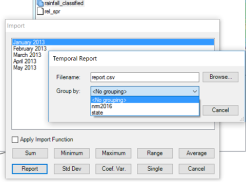
Figure 13 shows the process to add new layers from a time series to the MCAS-S workspace. Figure 14 shows how to use the time series import window. Repeat the process to add another layer using a different function.  

Figure 13 Flow chart to import time series data

1. Select the time series data you would like to include in your analysis, and drag it into the display workspace 
2. You will now see the Import window which lists the gridded data layers available within the time series. You can also see the metadata, tip or info file for time series data layers by clicking the Info button. See Figure 14
3. Select a time point by clicking on the listed grid or select multiple time points by clicking and holding down the shift key to select a group of grids, or the control key to select further individual grids for the group. 
4. From the Import window select; single (to bring in the selected time periods as individual layers), a standard function (to calculate a single new layer from multiple time periods), or combine a standard function with your own custom function. All time series functions are calculated on raw values.
   1. If you select Single from the import window then you be returned with the selected time periods as individual layers. No function will be applied. If you wish to save the layer right click to Export (section 8.1 Exporting). 
   2. If you select a standard function (SUM, MINIMUM, MAXIMUM, etc.), other than SINGLE you will be prompted to Save Layer. Type a filename and description which captures details of the dates chosen and functions that you have applied. Filenames should be short, unique, and only include numbers and letters. More details can be included in the Description field. The group field allows you to choose or create a folder to save your new layer in. For more information about writing and editing metadata see section 5.5.4 Metadata files. A new layer will appear in the MCAS-S display workspace expressing your chosen function for the selected grids. 
   3. If you check the Apply Import Function option check box you will then need to:
      1. Select a standard function, such as SUM, to combine the modified grids into the single output grid for display. This is will then open the Enter Import Function window.
      2. Use the Enter Import Function editor to enter a function (Figure 15). Syntax for the editor are shown in Table 1. This function will be applied to the raw data values of all selected grid layers (represented as {x}) and then the standard function (in this case SUM) is applied. For example, you could use an if statement to determine all the areas that meet a certain threshold (rainfall less than 10mm example shown in Box 3) and then SUM to see how many times that threshold is met across the time series. 
      3. Select Ok to apply the function. You will now be prompted to Save Layer. Type a filename and description which captures details of the dates chosen and functions that you have applied. Filenames should be short, unique, and only include numbers and letters. More details can be included in the Description field. The function is automatically entered in the Lineage field in the .tip or info file as shown in the save layer window. The group field allows you to choose or create a folder to save your new layer in. For more information about writing and editing metadata see section 5.5.4 Metadata files. A new layer will appear in the MCAS-S display workspace expressing your chosen function for the selected grids.
5. Check your new layer and the metadata (using the Info button on the interface panel). It is very important to correctly record processing details for future use. 

5.1.3.3 Apply functions to time series data

You can apply standard functions or combine a standard function with your own custom function, to generate a new data layer from time series data using the Import window. The options you can choose on the standard functions are:

• Sum – returns the addition of the values for each cell from the selected grids
• Minimum —returns the lowest value for each cell from the selected grids
• Maximum—returns the highest value for each cell from the selected grids
• Range—returns the difference between the maximum and minimum values for each cell (absolute variation) from the selected grids
• Average—returns the mean for each cell from the selected grids
• Standard Deviation (Std Dev.)—returns the standard deviation for each cell based on the selected grids
• Coefficient of Variation (Coef. Var.)—returns the coefficient of variation for each cell based on the selected grids.
• Single—returns the values as individual layers from each time period selected in the import window.

Apply Import Function— a custom import function can also be applied to time series data and combined with the standard function (except Single) shown on the time series data import window. Examples of syntax are shown in Table 1.

Figure 14 How to use the time series import window

Note: Time series data dragged from the Primary Input Data menu can be imported as individual datasets (Single option), or as a function of the selected datasets (Sum, Minimum, Maximum, Range, Average, Standard Deviation or Coefficient of Variation) with any required modification to the input data layers completed using the Apply Import Function option. To see the metadata for the time series use the Info button.

Figure 15 Apply a custom function to time series grids

Note: Selecting Apply Import Function and entering a manual function will modify each of the time series data layers selected BEFORE they are combined using your chosen standard function. In the example above, the NDVI (Normal Difference Vegetation Index - plant greenness) is multiplied by 0.0001 to account for the multiplication factor in the supplied data and return the values to the expected range (-1,1). And then the maximum NDVI is calculated for the 4 summer periods using the Maximum function. The function is then automatically entered in the Lineage field in the .tip or info file as shown in the save layer window. 

Table 1    Syntax examples for time series Enter Import Function editor

Syntax	Description
pow ({x}, 2)	For each import layer returns raw values to the power of 2. A standard function (e.g. SUM) is then applied to combine the layers.
exp ({x})	For each import layer returns the exponential of the raw values. A standard function (e.g. SUM) is then applied to combine the layers.
log ({x1})	For each import layer returns the base 10 logarithm the raw values. A standard function (e.g. SUM) is then applied to combine the layers.
iif ({x} > 20, 1, 0)	For each import layer returns a value of 1 where the raw value is greater than 20 and a value of 0 where raw values are equal to or less than 20. A standard function (e.g. SUM) is then applied to combine the layers.
min({x})	For each import layer returns the minimum value.  A standard function (e.g. SUM) is then applied to combine the layers.
max({x})	For each import layer returns the maximum value.  A standard function (e.g. SUM) is then applied to combine the layers.

Box 3    Where to live—applying a time series function

In this example we wanted to find areas which have summer plant growth (and exclude areas of bare soil which may be dry and dusty). Normalized Difference Vegetation Index (NDVI) provides a measure of plant greenness. We would like to group the expected NDVI values into four classes:

 

• > 0.5 healthy vegetation – most suitable
• 0.2-0.5 less healthy vegetation – less suitable
• >0-0.2 no vegetation growth (likely bare) - unsuitable
• - 1 to 0 (clouds or surface water) - unknown 

NDVI data was provided multiplied by 10,000 to enable the data to be stored as a smaller integer file without losing detail. This means that NDVI data have a much larger range than we are expecting. The custom function applied at Figure 15 returned the NDVI to the expected range for all selected time periods and then calculated the maximum value. 

If instead we had wished to COUNT the number of periods where NDVI was healthy (greater than 0.5 or 5,000 in the original data layers) we may have chosen a function iif ({x}<5000,1,0) to assign a value of 1 to pixels with NDVI above 5,000. Then the standard Sum function could be used to count the number of times this occurred for all the layers selected from the time series. The result would then be a layer with pixels ranging in value from 0 to 4 (or class 1 to 5) representing the number of periods that NDVI was above the threshold. 4 represents consistently healthy vegetation. 

5.2 Overlay data

What are overlays?

Overlays are lines or points (such as roads, towns, and coastline) that can be added to a primary data layer to provide context. Overlay data are stored in the \Data\Overlay folder.

Steps to display overlays

To select and display overlays:

1. Expand the Overlay drop-down menu (Figure 16). 
2. Check the box next to as many overlays as desired.
3. Change overlay colours. To change the overlay line or point colour from the default (black) click on the colour box for the layer in the drop-down menu. You can then select a new colour from the colour palette. Different colours are useful to distinguish multiple overlays.

Why are only some overlay points labelled?

MCAS-S can display labels for points such as cities and towns. The number of points and labels displayed depends on the size and zoom level of the data layer being viewed. For example, when a data layer is small and towns are selected only major cities may be visible, but as you enlarge the window or select a region mask, towns with smaller populations may become visible. To turn point labels on and off or modify other settings see section 5.5 Preparing your own data.

Can I include overlay data in my analysis?

Adding an overlay will not change or affect the data or the results of a multi-criteria analysis, but will provide lines, borders, or points to assist interpretation of the map.
To include information from overlay layers in the analysis you can bring these layers in as a grid of distance from points or lines. To create a layer from a point or line overlay to use in the analysis click and drag the overlay layer into the workspace. For more information see section 5.5.1.2 Distance from point or line overlays

Figure 16 Point and line overlays

Note: Figure shows a continuous primary data layer (elevation) with a point overlay (capital cities) and line overlay (state boundaries). Overlays are added by checking the box in the overlay dropdown menu. Overlays only provide context and cannot be used in analysis.

5.3 Mask data

What are mask data?

Masks can be used to select specific areas for analysis and reporting. Mask data are gridded raster data like primary categorical data. Find available mask data by clicking the Mask Icon at the top of the MCAS-S workspace and selecting from the available folder icons. Mask data requires either an associated text file or class labels identified from a data field. Mask data can either be saved in the \Data\mask folder or also in the /Data/Primary folder. To see more information about preparing mask data in the appropriate format see 5.5.3 Preparing mask data. You can use masks to display only the data for a selected region (for example, zoom in to a catchment or bioregion) within the map in the display workspace. When masks are selected, masking applies to all functions and processes carried out in an MCAS-S project.

Do I need to apply a mask to make a report?

No — You can create a report using any set of regions in the masks drop-down menu, even when an MCAS-S project is not masked. Reporting is covered in section 8.2 Reporting.

Steps to apply masks

To apply a mask:

1. Expand the Mask drop-down menu and check the box next to the regions required (see section 5.5 Preparing your own data for installing mask data layers). 
2. Choose whether to maintain the full data range, or update your data range for the masked view, using the Mask interface panel.
   1. Mask view only 5.3.1 Mask view only (default) maintains the data range for the full extent of data layer as you zoom in, or
   2. Mask View and Data 5.3.2 Mask view and data reclassifies the data to match the smaller extent and reduced data range of your selected masks.
3. To apply more than one mask:
   1. Once you have selected one mask hold down the shift key to select further masks. 
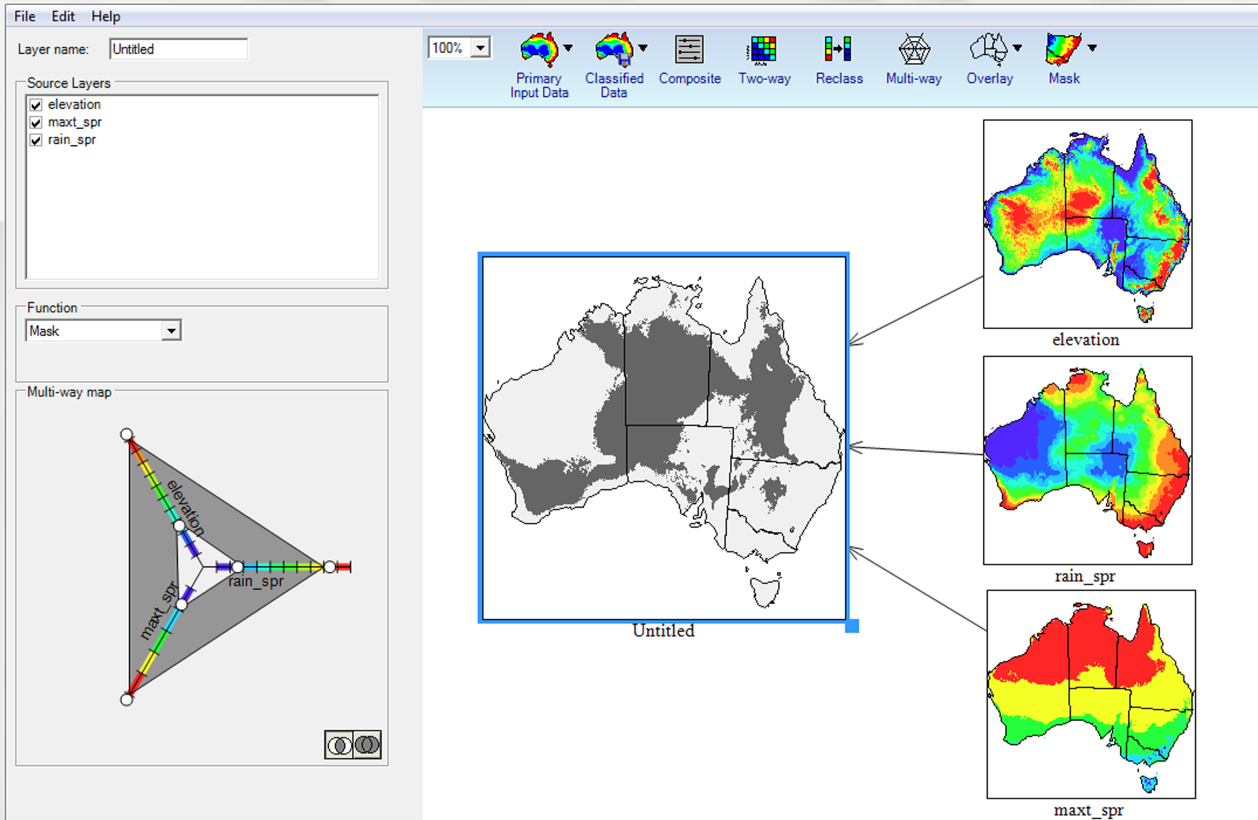
   2. Choose whether you would like to display an Aggregate or Intersection of the two or more selected masks using the Intersect and Aggregate mask option buttons at the base of the Mask drop-down menu (Figure 17).
      1. The aggregate mask (default option) is like an OR function, showing pixels which occur in any of the regions selected,
      2. The intersection mask is like an AND function showing only the pixels which occur in all of the selected regions. 

Figure 17 Intersect and aggregate mask option buttons

Options to remove masks

To clear masks from showing in your project you can either

• Deselect each selected mask individually by clicking in the check box – this option is useful if you only have one mask selected or if you wish to remove a particular masked region but keep another mask active. 
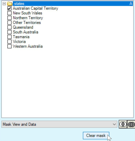
• Clear all masks and return to the full view using the Clear mask button – this option will remove all masks and return to the full view. This also useful to return to original workspace pan and zoom.

Figure 18 Clear mask to remove all active masks

5.3.1    Mask view only

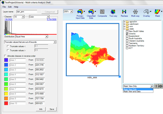
Select Mask View Only from the drop-down menu in the Mask interface panel to zoom all layers to the selected regions (Figure 19). Mask View only will not change the display and class allocation of the data it will simply restrict your layer view to the region (or regions) chosen. The values shown in the histogram still refer to the full extent of the layer even though the whole layer cannot be seen.

Figure 19 Example Mask View Only

Note: Figure shows annual rainfall data masked to the Victorian state boundary using the Mask View Only option

5.3.2    Mask view and data

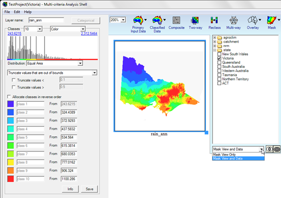
Figure 20 illustrates the Mask View and Data function. Only annual rainfall values specific to Victoria are displayed, and this is reflected by the changes in both the class allocation in the interface panel and in the display in the map window.

Previously, when mask view was selected, or a mask was not applied, the values in the classification ranged from approximately 136.5936 to 5,754.5806 (Figure 19). However, applying Mask View and Data function (Figure 20) changes these values to approximately 243.6215 to 2,312.5464 as applicable to Victoria only and not to the whole of Australia. 

Figure 20 Example Mask View and Data

Note: Figure shows the annual rainfall data layer, with view and data masked to the Victorian state boundary using the Mask View and Data option

5.4 Classified data

What are classified data?

Classified data are layers that you, or another MCAS-S user, create from an MCAS-S analysis. Any data layer that you create or modify and export as a new layer in MCAS-S will be saved into the Classified data folder. This includes New User layers (see section 5.6 Creating user layers) and overlay distance layers (see section 5.5.1.2 Distance from point or line overlays). It is particularly useful to export layers which you have customised or created using any of the MCAS-S analyses (two-way, multi-way, composite or user layer) to preserve the layers for future use and record details of the steps taken to create them. More information on combining MCAS-S data layers is provided in section 6 Step 3: Explore and combine data.

How do I make a Classified data layer?

Create classified data layers by exporting any open layer in the MCAS-S display interface. 

How do I add classified data to my MCAS-S project?

Once created, add these new layers to your project by selecting and dragging them from the Classified data drop-down menu.

5.5 Preparing your own data

You can create MCAS-S projects using your own input data layers. You will usually need to use GIS software to pre-process your own data to ensure it meets the MCAS-S requirements, which are set out in this section.

WARNING: To prepare data you will need GIS software, careful consideration of how your data will be used, correct folder structure, and consistent spatial referencing system and extent for all layers. 

Plan your new MCAS-S data

1. What the data will be used for? Your data can be any of the data types already discussed depending on how it is to be used. 
   1. for analysis – Primary (see 5.5.1 Preparing primary data)
   2. for context – Overlay (see 5.5.2 Preparing overlay data). Note overlay data can be included in analysis as distance to lines or points see section 5.5.1.2 Distance from point or line overlays.
   3. for reporting or restricting the view - Mask (see 5.5.3 Preparing mask data)
2. How will the data be presented?  
   1. Categorical – which attribute will be used to create the class values? (See 5.1.1    Categorical data and 5.5.1 Preparing primary data).
   2. Continuous – is there a numeric attribute value that can be used or is creating a metric value, such as minimum, mean or maximum, more useful? (See 5.1.2 Continuous data).
3. Ensure your data is spatially consistent
   1. Scale – choose an appropriate grid size for your primary and mask data. While MCAS-S can accept layers with different grid sizes it is important to consider how this may affect your data layer combinations. A maximum of 4000 x 4000 pixels is recommended for primary data layers when using the 32 bit software version (~1km grid for Australia). The 64 bit software can handle more, higher resolution, data layers. Very high resolution layers are likely to cause MCAS-S to run slowly or crash. This could be addressed by having several MCAS-S projects dealing with different regions.
   2. Referencing system – input data for use in MCAS-S MUST have a consistent spatial-referencing system, (that is, a common projection). For example, the gridded data layers from the sample project and the Australian national map layers available on the MCAS-S website are in Albers Equal Area projection using the Geocentric Datum of Australia 1994 (commonly referred to as GDA94),
   3. Extent– input data for use in MCAS-S MUST have a consistent spatial extent. Primary layers and mask layers must have common bounding boxes with the same north latitude, south latitude, east longitude and west longitude in order for MCAS-S to calculate correctly. For example, to prepare new data to use with the gridded data layers from the ready-to-use Australian national map layers available with MCAS-S version 3.2, match the extent of the new data with any of the ready-to-use layers in the Primary folder
4. What is the appropriate time period? – Data can be presented as a single time period or as a time series (5.1.3 Time series data and 5.5.1.1 Time series data)
5. How do you want MCAS-S to display and combine no data or missing data? Many data layers have areas of No data or missing data. Make sure to choose an appropriate option for No data to suit your MCAS-S analysis. Consider that you may have different types of No data in a primary layer. For example there may be locations outside of the extent or scope your study area and areas where data was unavailable, unreliable, or confidential. Deciding how to combine layers which include No data is discussed further in section 6.4 Combining data (composite development). For an MCAS-S analysis you may:
   1. Option 1)    Assign areas of No data to -9999. MCAS-S recognises and treats the value –9999 as ‘No data’ or missing values. MCAS-S shows areas of -9999 using grey hatching. -9999 is the recommended value to assign to areas of missing data inside your reporting region, or area of interest. The advantages of assigning No data areas to -9999 are that you can: report on the area of -9999 in any input layer or composite, edit areas of -9999 using the user layer tool when expert opinion or new data becomes available, choose whether to mask out areas of -9999 leaving a hole in an combined data layer or allow other layers to fill in these areas. 
   2. Option 2)    Leave areas of No data blank or No data. No data or blank areas are recommended to indicate areas outside of your area of interest for example outside of the coastline of Australia. MCAS-S will show these areas as blank white space. No data pixels will be excluded from reports. You can choose to leave these areas as blank (default) or fill these areas with other layers which have values for these pixels in a composite. When exporting a layer from MCAS-S, blank no data areas will be assigned a value of -999. 
   3. Option 3)    Assign a category for No data. In categorical data layers you may choose to assign any value for No Data and label this accordingly. Assigning a value other than -9999 to missing data may have implications for classifying and combining data layers and should be carefully labelled and described in the .tip file.  
6. Correct folder structure – your data must be saved alongside the MCAS-S project in the Data folder structure shown at Figure 21.

The following sections contain more specific information to help you process data for use as primary (5.5.1 Preparing primary data), time series (5.5.1.1 Time series data), distance from point or line overlays (5.5.1.2 Distance from point or line overlays), overlays (5.5.2 Preparing overlay data) and masks (5.5.3 Preparing mask data) and to prepare metadata to accompany each data layer (5.5.4 Metadata files) . 

Data conversion documents for use with the GIS software programs such as ArcGIS are also available on the MCAS-S website.

Your pre-processing is complete when spatial data inputs are located within the project file structure and are ready for use in MCAS-S drop-down menus under the headings Primary Input Data, Overlay and Mask as shown in Figure 10.

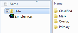
Figure 21 The Data folder structure required for MCAS-S projects

Note: The data folder must be saved alongside an MCAS-S project and contain the folders Primary, Classified, Mask and Overlay as shown 

5.5.1    Preparing primary data

Do I need to include Primary data?

Yes — you need Primary data to do any analysis in MCAS-S. Primary data are raster data. See section 5.1 Primary input data

Steps to prepare new primary data

1. Convert data to a raster data format such BIL, binary float-point file, Arc GRID or Geotiff. GIS systems use two types of data—raster and vector. For raster data, representation of objects is based on the elements of a matrix, given as grids or pixels. For vector data, representation is based on distinct points described by their coordinates and relations.
2. Ensure data is in a numerical value field. 
   1. Continuous data will already have a numerical value field. Consider converting the values to integers to reduce the size of the layer file. 
   2. Categorical data requires numbers and names: Convert categorical data (that is, data expressed using classes such as states and territories) into a numeric code. There are two options for including category names:  
      1. Option 1)    Category names in a text file: Ensure your categorical layer has a single value field that contains the numeric code. Create a text file with the same name as the raster. This file will list “value” “label” and then a list of values and corresponding labels (for example 1=New South Wales; 2=Victoria etc.) using the same structure as the Mask text file (Figure 26). Save the text file in the same folder as the raster.
      2. Option 2)    Category names as a field: MCAS-S version 3.2 can read labels and numerical categorical weights from fields in the raster data layer of Geotiff and ASCII files (not ESRI grids). In order to use this option you need to ensure that the .tip file of your categorical data layer has each of these columns (Figure 22):
         1. CategoryValue: name of the field containing numerical values e.g. ‘CategoryValue: Value’
         2. CategoryLabel: name of the field containing the labels e.g. ‘CategoryLabel: Label’
         3. CategoryWeight (optional): name of the field containing numerical categorical weights or ranks indicating the order by which MCAS-S should classify the data e.g. ‘CategoryWeight: Weights’
3. Create associated metadata, info or .tip files if not done so already (section 5.5.4 Metadata files)
4. Save data, .tip, and .txt files in the project directory \Data\Primary. 

Figure 22 Assigning field as category names for categorical data

5.5.1.1 Time series data

Do I need to include time series data?

No — if you have consistent information for multiple time periods you may wish to package this as a time series for use in MCAS-S. Time series data is a type of primary data for analysis (see also section 5.1.3    Time series data). Packaging data as a time series orders or stacks the layers by date and allows you to apply time series functions or reports.  

Steps to prepare new time series data

1. Ensure time series data is consistent with other primary data
2. Store as a stack of raster files in the appropriate format 
   1. in a separate folder 
   2. created within the \Data\Primary folder. 
3. Name the time series layers correctly - for MCAS-S to recognise the data as a time series, each component dataset needs to contain a string of either six digits or eight digits preceded by an underscore; six digits is assumed to be YYYYMM and eight digits is assumed to be YYYYMMDD. For example, ‘rain_198001’ would be a time slice of rainfall for January 1980 and ‘rain_20051231’ would be a time slice of rainfall for 31 December 2005. Note that once you have chosen a name for a time series, each data point must have this prefix before the date.
4. Decide whether to use raw or classified values. 
5. Save an info .tip file relating to the whole time series data stack within the \Data\Primary folder data but OUTSIDE the folder containing the time series data layers. 

5.5.1.2 Distance from point or line overlays

To use overlay data in your MCAS-S project as an input layer rather than a contextual layer it must be converted to a raster. See section 5.2 Overlay data. MCAS-S can create a raster of distance from the points or lines contained in an overlay layer.

Steps to include overlay data in your analysis

1. Add at least one primary input layer to your MCAS-S workspace. This layer will be used as a mask providing the cell size and location boundaries for the new layer that you are about to create. 
2. Click on the overlay in the overlay menu, and drag the layer into the MCAS-S workspace. The New Distance Layer window will pop up.
3. Select a mask. The New Distance Layer window (Figure 23) requires you to select a mask from the layers already open in the MCAS-S workspace that you wish to model your new layer on. The mask determines the cell size and included locations for the new layer. Click ‘Ok’.
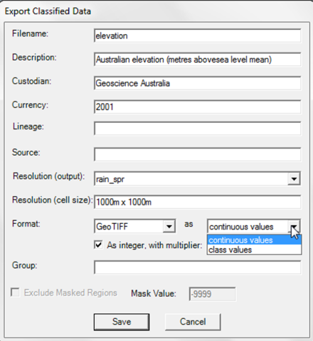
4. Choose a filename, Description and group. In the Save Layer window (Figure 24) type a short filename, a detailed description of the layer, and the folder or group name under Classified where you wish the data layer to be saved. Press Save.  
5. MCAS-S has now created a gridded data layer showing the Euclidian distance (based on number of pixels) of each cell to the overlay lines or points (Figure 24) in the workspace. This layer is also saved in the classified data folder and can be used as a primary data layer in MCAS-S analysis. 

Figure 23 New Distance Layer window

Note: To create a distance to capital cities, click and drag the capitals point overlay into the workspace. You need to choose a mask to set the cells size and any areas to be excluded from the new layer. 

Figure 24 Save Layer new distance from a point overlay

Note: Once an overlay is dragged into the workspace and the mask set (Figure 23) the Save Layer window will appear. Enter the details and click Save and the layer will show in the workspace. In this image the histogram on the left-hand side interface panel in the figure shows the approximate minimum and maximum number of pixels from a capital city. 

5.5.2    Preparing overlay data

Do I need to include overlay data?

No — overlay data is optional – MCAS-S can display vector polygons, lines or point data (with or without labels) for as contextual information however these are optional. For more information about overlays see section 5.2 Overlay data.

Steps to prepare new overlay data

1. Save overlay data as a vector file such as an ESRI shapefile or coverage with consistent referencing system and extent to the rest of the data for the project.
2. Save overlay data in its own folder in \Data\Overlay folder in the project directory. Each overlay file must be placed in an individual folder in the overlay folder for example\Data\Overlay\Cities. The names of the overlay folders will be displayed in the Overlay drop-down menu in MCAS-S.
3. Point overlays must have an associated text file. The text file for point overlays describes how to display the point. Ensure that:
   1. The text file has the same name as the overlay folder
   2. The text file is saved under \Data\Overlay rather than in the individual folder with the actual overlay dataset 
   3. The text file contains the fields below. An example of a text file for a point dataset is shown in Figure 25. Note that some of the above settings may be overridden depending on the sizes of layers in the MCAS-S workspace. If some points appear to be missing, try maximising the size of layers to ensure desired points and/or labels are displayed. If this does not work, the pointFilter and nameFilter settings may need to be increased.
      1. data = value field name. This is the name of the field that contains the values that determine the order in which points will be displayed. This could be an existing field or you may need to create it with GIS software. Larger numbers will display first, with smaller numbers progressively displaying as the data layer is enlarged, so if you chose to display city points by a population field, a city with 2,000,000 will display before a city with 100,000. When creating a new data display field, give higher values to points which are to display first.
      2. name = label field name. This is the field containing labels for the points.
      3. pointFilter = 1 – 1000+.  This is a scale starting at 1 that controls the number of points displayed. If you enter the number 1, only the most important points [as determined by a large value in the data field] will be displayed. To display all points, choose a large number such as 1000. Note that depending on the number of points in the layer, the pointFilter value may need to be adjusted several times to display the desired number of points.
      4. nameFilter = 1 – 1000+ Similar to the pointFilter, this is a scale that controls the number of labels displayed. If you enter the number 1, only a small number of labels will be displayed. To display all labels, choose a large number such as 1000 [this may need to be larger depending on the number of points]. It may be advisable to set the name filter lower than the point filter so labels do not become too crowded
      5. showName = true (labels display) or false (labels do not display).

Figure 25 Example of text file information for point overlay data

Note: In this example, the field containing the data for displaying the points is called ‘OBJECTID’, the label field is ‘NAME’, the filter for displaying points and labels is 1 (fewer points and labels will display as the layer is minimised) and the display of labels is turned on (‘true’).

5.5.3    Preparing mask data

Do I need to include mask data?

No — Mask data, raster data that define the geographic limits for analysis and reporting is optional. However, you cannot run Report by region unless you have Mask data loaded. You can use masks to show or report on information within an area of interest, or to generate a report comparing values within different regions. See section 5.3 Mask data Mask data require a numerical field and matching labels to be used in MCAS-S.

Can I use primary data layers as masks?

Yes – Primary categorical data layers can be used as masks by MCAS-S version 4. Figure 27 shows Land use data displaying as a Mask dropdown list and also as a primary layer in the workspace. Being able to use the same data for analysis or reporting may reduce redundancy and decrease the size of your data pack. To enable MCAS-S to recognise primary layers as available as masks you need to add an extra line to the .tip, info or metadata file: CategoryAsMask: TRUE. Figure 28 shows an example tip file for the land use data layer including this field. 
Add CategoryAsMask: TRUE to .tip files for categorical raster data saved in the primary data folder if you wish to use these layers as BOTH a primary layer and a mask without needing to duplicate the layer in the mask data folder. 

Steps to prepare mask data

1. Use the correct format. Import or prepare gridded mask data files in BIL, binary float-point file, Arc GRID or Geotiff raster formats. Mask data layers must conform to the primary data extent. 
2. Choose or create a numerical field. Mask data use a numerical field matched to labels to report or restrict the project view. For example in the States layer, 1 = New South Wales etc. 
3. Choose or create labels for the mask classes. Mask data layers require labels which match to a numerical field. MCAS-S can recognise labels saved as: a text file accompanying the mask data layer, or labels from a field in the data layer identified in the .tip file. The labels display in the Mask drop-down menu on the MCAS-S interface (Figure 26).
   1. Labels from text file: Include a text (.txt) file with the same name as the mask file in the Mask data folder. This file needs to list the numerical code and the associated label for each class. The left window in Figure 26 shows the state mask with labels and grid values from the state text file. The right window shows the corresponding list of states from the Mask drop-down menu on the MCAS-S display workspace.
   2. Labels from a field: Specify a data field containing the mask labels using the tip file (section 5.5.4 Metadata files) by including the entries: CategoryLabel: for the labels and CategoryValue: for the associated class numbers. 
4. Save data to be used as masks either 
   1. in the project directory \Data\Mask. or
   2. in the project directory \Data\Primary ensuring the .tip file contains Category as mask: true
5. Check the .txt (label) and .tip (info) files are formatted correctly to allow MCAS-S to identify the layers as a mask and read the class labels.

Figure 26 Mask data text file contents

Figure 27 Mask data loading from the primary data folder

5.5.4    Metadata files

What are Tip or info files?

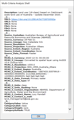
Metadata files are called tip files in MCAS-S. You should create tip files for each new layer that you add to MCAS-S. Tip (.tip) files contain extra information about the data layer to ensure that the layer is used and interpreted correctly (Figure 28). 

What if there is no Info button?

No Info button in the interface panel when a data layer is active means:

• .tip or metadata file has not been created for the layer, or
• the .tip or metadata file has a different name to the layer.

It is advisable to create and edit .tip files for each layer in your project to ensure they are current and correct.

How can I make or edit tip files?

Some MCAS-S functions that create a new MCAS-S data layer will prompt you to create tip file by typing layer details. You can also view, create and edit tip files outside of MCAS-S using a text editor. To create a new .tip file with the correct structure you can copy the structure of an existing .tip file and rename it to match your data layer. The text should be specific for the dataset. Tip files should be saved beside primary data layers with the same name as the primary data layer. Tip files for time series data layers should be saved beside the time series folder with the same name as the folder. Even though it is not possible to view tip files for overlay and mask data in the MCAS-S software, tip files are recommended for any data that you add to your MCAS-S project. You can also use tip files to direct MCAS-S to read labels for categorical and mask data layers from a field in the data file. 

What information do Tip files include?

Tip files can include the following fields:

• dataset name—short name which displays when mouse hovers over it
• description—longer data name including more information such as units if applicable
• custodian—organisation that owns the data
• currency—year (for example, 2006)
• resolution—grid size of the raster data; layers in the sample project have been provided at a resolution of 1000 m x 1000 m
• lineage—processing completed on the data (for example, source, calculations, software/ commands used)
• URL—a hyperlink to a website where more detailed metadata may be found. Note that accepted formats for hyperlink are http://websiteaddress.com or https://websiteaddress.com
• file—a link to another file saved alongside the data layer that contains more detailed metadata. MCAS-S can recognise files with extensions .doc .docx .rtf .mht .pdf. To reference another file use the format file: myfile.doc
• CategoryValue: (categorical or mask data) where a categorical dataset contains more than one field you must specify the name of the numerical value field e.g. Value. This field is the numbers that relate to the labels. For example for States the field “Value” contains a 1 for New South Wales. 
• CategoryLabel: (categorical or mask data) the name of the field containing labels e.g. Label
• CategoryWeight: (categorical data-optional) if you wish to use the numerical categorical data classification option (section 6.2.2    Classifying categorical data) this is name of the field containing numerical categorical weights or ranks indicating the order by which MCAS-S should classify the data. You will also be able to select other fields to weight or rank the data layer by from a drop down list once the layer is open in the in the MCAS-S software.  
• CategoryAsMask: TRUE (categorical data – optional) add this field to categorical data if you wish to save this in the primary data folder allow this to be used as either or BOTH a primary layer and a mask see also 5.3 Mask data. 

You can also add other custom fields to your tip files.

Figure 28 Tip or Info file window

Note: To access information in a .tip file for a selected primary input data layer clicking the Info button on the left-hand interface panel or in the Import window for time series layers. 

For continuous data layers do NOT include headings CategoryValue, CategoryLabel, CategoryWeight or CategoryAsMask in the tip files or MCAS-S will display this data as categorical by default.

5.6 Creating user layers

What is a User layer?

You can edit any layer in an MCAS-S project display workspace (except multi-way layers) to create a new user layer. Creating a user layer is a way of capturing expert knowledge where other data may be incomplete or unsatisfactory, and incorporating this knowledge into an MCAS-S project. New user layers are based on the classes of an existing layer. Raw values are not shown in new user layers. While pixels can be painted or filled with any class colour, the order and number of classes are fixed once the layer is created. For this reason, it is important to make sure that your layer is appropriately classified before creating a new user layer.
Steps to make a new user layer

Layers can be created from scratch, with only the boundary of an existing layer used, or edits can be made to an existing layer. To create a user layer:

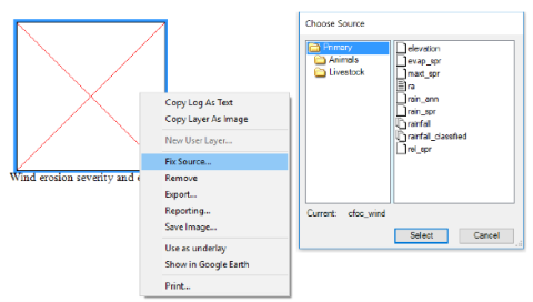
1. Right-click on a layer in the display workspace and select New User Layer. 
2. The New User layer dialogue box will appear. Fill the spaces to give the new layer a filename, description and so on. 
3. Choose the resolution (output): this field shows the data layer that will be used as a template to set the cell size for the new layer. Your chosen layer is the default, however you may change this to any other layer open in your project window (except multiway layers). The resolution (cell size) will automatically update depending on the cell size of the Resolution (output) layer. You cannot change the cell size of the new layer by typing in the Resolution (cell size) field but typing in this box will change the text in your metadata (.tip) file for the new layer. 
4. Enter the Group field if you wish to save the new layer to a new or existing group (folder) or leave the field blank to save directly under the Classified Data (Figure 29). 
5. Select data to include in the new user layer using the Data drop-down menu. Choose one of the following options to determine what you want the layer to look like before you begin editing:
   1. Option 1)    copy the existing layer, Your new layer will have the same number of classes as your original layer (which cannot be changed),
   2. Option 2)    set the layer to –9999. This will create a new blank layer ready for editing, you can now choose the number of classes for the new layer (this cannot be changed later). 
   3. Option 3)    set the layer to one of the existing classes. This will fill all pixels in the layer with the colour of the class that you have chosen regardless of what class they show in the original layer. You can choose the number of classes for the new layer (this cannot be changed later).
6. The new layer will appear in the workspace (and is saved under the Classified data folder see section 5.4 Classified data). To view the metadata information, click on the Info button on the interface panel see section 5.5.4 Metadata files.

Figure 29 New User Layer settings window

Steps to edit a new user layer

Once your new user layer is in the MCAS-S project workspace you will see an Edit button in the left hand interface panel. To edit your new user layer:

1. Click on the Edit button in the interface panel to open an Edit window (as shown in Figure 30.)
2. Choose where to allow editing. Use the Clipping drop down list below the layer display in the editing window to choose which areas you may edit: 
   1. Option 1)    clip out no data—this option is the default setting; you will be able to edit areas with a class value or set to –9999. ‘No data’ areas, or areas outside the extent of your previous data layer, cannot be edited (for example you may not be able to colour outside the coast of Australia).
   2. Option 2)    no clipping— all pixels in the new layer may be edited. You can now apply colour anywhere within the editing window even outside the extent of the previous data layer (for example outside the Australian coast). 
   3. Option 3)    clip to –9999—only areas set to –9999 can be edited. This option is useful for filling ‘holes’ to incorporate updated data or expert opinion especially in workshops.
3. Edit the layer: You can edit the layer by painting with a brush, and / or filling whole regions
   1. Option 1)    To paint areas of the layer, select a brush size using one of the black squares to the left of the layer, and select a class colour from the options at the top of the layer. The available colours refer to the classes in the original layer. Areas on the map can be edited by either left-clicking or clicking and dragging to edit larger areas. 
   2. Option 2)    To colour areas based on regions, click the Fill button, The Fill by Mask window will open (Figure 30). Choose a Mask region and assign class numbers to one or more of the regions using the drop-down menus (for an example comparing edits made using paint and the fill options, see Figure 31).
4. Save or discard your edits regularly. To save your edit use the Save button. To undo any edits click the Cancel button. Note that clicking the Cancel button will erase all unsaved changes made during the editing session.

Figure 30 Editing a new user layer

Note: The figure shows editing a new user layer based on Elevation. Edits can be made using the paint functions or by filling whole mask regions with a value (as shown in the open fill window).

Figure 31 Using the paint and fill tools to edit a user layer

Note: Edits have been made to central Australia (blue), parts of Western Australia and New South Wales (red in south-west WA and red square in western NSW) using the paint functions, and Victoria and Tasmania have been re-assigned values for the whole state using the Fill tool (as can be seen when compared to the original layer)
This section outlines how to assemble data and how to bring data layers into the MCAS-S display workspace, ready for use. The next section outlines how these data layers can be classified, compared and combined to explore the data.

6    Step 3: Explore and combine data

This section describes how to set up the MCAS-S workspace, classify the data, and explore simple relationships between data layers. You can compare and combine primary data layers in MCAS-S by assigning raw data into classes and working with these classes. 

6.1 Setting up the MCAS-S workspace

There are many options for optimising your view of the MCAS-S workspace and your data layers. Use the View menu, the scroll or slider bars, keyboard shortcuts and mouse or touch screen. To return to the original view use reset view on the View menu and or Clear Mask from the Mask icon. 

Figure 32 Zoom, pan, and move around workspace

6.1.1    Moving around the workspace

To move around the workspace:

1. Scroll: use the slider bars at the bottom and right-hand side of the workspace, or 
2. Mouse pan: hold and press the spacebar while clicking and dragging somewhere on the workspace.

To view only the workspace, or to return to the interface panel view, click the full-page icon on the right hand size of the workspace (see Figure 7).

6.1.2     Move or resize data layers 

You can move, align or resize single or multiple data layers by:

1. Select the layer, or layers to be moved or resized: Click on a single layer or hold the shift key while clicking to select multiple layers. Selected or active layers are shown by a dark blue border
2. To move: 
   1. Option 1)    drag to a new location using the mouse, or
   2. Option 2)    align the selected layers to top, bottom, left, or right by selecting these options from the left-hand interface panel when multiple layers are selected. 
3. To resize: 
   1. Option 1)    click the bottom right-hand corner of the layer with the mouse and drag to the desired size, or 
   2. Option 2)    select “resize to smallest” or “resize to largest” from the left-hand interface panel when multiple layers are selected. 

6.1.3    Remove layers

To remove any layer from your MCAS-S workspace right click and select Remove. Remove multiple layers at once by clicking on the layers to be removed while holding down the shift key then righting click and selecting remove.
Remove deletes the active map window from the display workspace. Removing a layer from the workspace will not delete the underlying data. The layer can be added back into the workspace but the classification may be lost. 

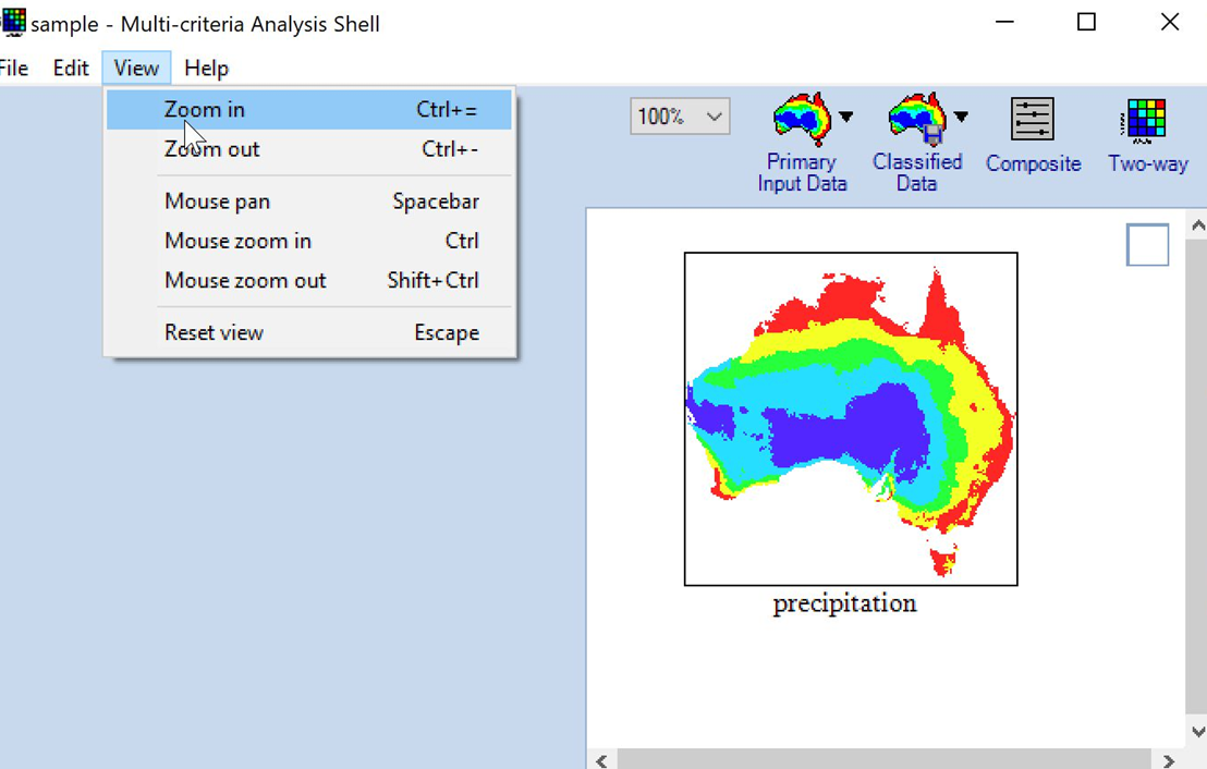
6.1.4    Zoom options

There are multiple zoom options (table 2): you can zoom in and out of the workspace to fit more layers in view, expand a single map layer to full screen, zoom in on (or out) location in all map layers simultaneously.  To adjust the magnification of the workspace

1. Zoom in on the workspace  
   1. hold the control key and click anywhere in the workspace, or  
   2. select a larger magnification (such as 200%) from the zoom drop down list in the left corner of the MCAS-S functions toolbar.  
   3. go to the View menu and select Zoom in. The view menu also shows the keyboard shortcuts.
2. Zoom out of the workspace,  
   1. hold the control and shift keys and click anywhere in the workspace, or  
   2. select a smaller magnification (such as 50%) from the zoom drop down list in the left corner of the MCAS-S functions toolbar.  
   3. go to the View menu and select Zoom out. The view menu also shows the keyboard shortcuts
3. Expand a single map layer to full screen, double click anywhere in the layer. Press Esc to return to normal view. 
4. Adjust the magnification within the data layers (all layers will move simultaneously)
   1. Zoom into all data layers  
      1. cnrtl +Alt + left-mouse-click
   2. Zoom out of all data layers  
      1. cntrl + Alt + shift + left mouse click 
   3. Pan around all data layers 
      1. Control + Alt + space bar + mouse click + mouse move

Table 2.  Zoom and pan shortcut keys

Zoom affects	Function	Hot keys & mouse action
Workspace	Zoom in	Ctrl + left mouse click
Workspace	Zoom out	Ctrl + Shift + left mouse click
Workspace	Pan	Spacebar + left click on mouse drag Middle mouse button + drag
Single layer	Full screen	Double click
Single layer	Remove from full screen	Esc
All layers	Zoom in	Ctrl + Alt + left-mouse-click
All layers	Zoom out	Ctrl + Alt + Shift + left-mouse-click
All layers	Return to full extent	Mask dropdown menu – clear mask
All layers	Pan	Ctrl + Alt + space bar + move mouse
Reset	All  (pan and zoom)	Esc

6.2 Classifying data

Do I need to classify my data layers?

Yes — MCAS-S analyses work by combining and or comparing classified data layers. 
Almost all of the classification options in MCAS-S assume that the data is arranged in such a way that ‘suitable’ occurs at one end of the scale of values, while ‘not suitable’ occurs at the other end. In the example ‘Location of where to live’ all inputs will be classified from low to high risk of degradation.

Steps to classify data layers

1. Choose a consistent classification system for your project: When classifying data, it is important to use the same classification system for all data. For example, all of the data being classified from ‘suitable’ to ‘not suitable’, or from ‘high’ to ‘low’, or from ‘good’ to ‘poor’, in terms of the objective. You can then assign colours so that, for example, blue classes always denote ‘not suitable’ and red classes always denote ‘suitable’. This consistency will ensure that input layers are compared and combined using the same classification system. The default classification system in MCAS-S shows areas of high values in red and areas of low values in blue.
2. Assign classes to continuous and categorical data as described in section 6.2.1    Classifying continuous data and 6.2.2    Classifying categorical data below using your consistent system. In the default blue to red classification, you should assign areas of most interest to the red class.
3. Record your classification: you may wish to save the new classification for your data layers to maintain the classification if you remove and re-add a layer to the workspace. You can save your classification for a data layer by:
   1. Using the Save button on the left-hand interface when that layer is active. WARNING: using the save button to save the class settings for a data layer makes them the default display settings for that layer in the current project and other projects which use the same data folder, or 
   2. Export and save a copy of the data layer with your classification applied (section 8.1 Exporting).

Data layers that don’t fit the classification system

Sometimes a moderate value may be the most suitable value with extreme values being less suitable, or data has previously been classified to meet another objective. The reclass tool described in section 6.2.3 Reclassifying data to a new order allows more flexibility in assigning classes to the most appropriate order for analysis.  

6.2.1    Classifying continuous data 

Steps to classify continuous data layers including time series

1. Understand the data layer: It is very important to ensure your classification is appropriate and meaningful for the data and the project. Information about the layer is shown in the left-hand interface panel (Figure 33). There is also a histogram which shows the data distribution and approximate maximum and minimum values. For more information about the layer, such as source, units and currency, click on the Info button to bring up its metadata. If the Info button is not displayed, then there is no metadata (.tip file) for the layer. 
   1. If you want to classify this layer as a categorical data layer instead of a continuous layer, use the Categorical button on the interface panel and proceed using instructions in 6.2.2 Classifying categorical data
2. Choose the number of classes: each primary data layer can be classified in 2 to 10 classes. 5 classes are the default.
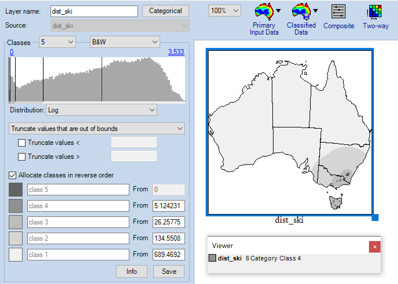
3. Consider reversing the class order: Are you most interested in the largest values for this continuous data layer? If not, you may need to reverse, or reclassify your continuous data. The default display for continuous primary data layers in MCAS-S is to assign the largest values to a class of most importance shown in red, and the smallest values to a class of least importance shown in blue. This becomes particularly important when combining data layers into composites. For example, high values may be preferable for some layers in terms of the overall question (such as high median income in the ‘Where to live’ example) whereas low values may be preferable in another layer (such as close to ski fields). Reversing class allocation means that layers can then be classified using the same colour scheme.
   1. To reverse the order of the class colours (to assign more importance to lower values): Check the box labelled Allocate classes in reverse order box in the continuous Primary Input Data interface panel. 
   2. To place most importance on a moderate, or specific value, in a data layer use the reclass tool (6.2.3 Reclassifying data to a new order) or consider whether using a two way, multiway, or function composite to combine your data layers may be appropriate. 
4. Choose the way that the values are assigned to classes: You can classify your continuous data layers into classes using: Equal interval, Equal area, Log, Standard Deviation, Natural Breaks or Custom (user-defined) classification under the Distribution drop-down menu. 
   1. Equal interval groups the data into classes with regular value steps regardless of their distribution. 
   2. Equal area allocates the same number of data points to each class (Figure 33). 
   3. Log allocates classes in a logarithmic scale by value. Given a set of values from x0 to x1, the range of the values is x1 minus x0. To find a log classification for n classes, MCAS-S determines the nth root of the range and uses this value as the base of the log. For example, a set of values from 0 to 1000 has a range of 1000 (1000 minus 0). If it were classified into three classes, the cube root would be 10, leading to splits of 10 and 100. If it were split into five classes, the fifth root would be ~3.98107, leading to splits of ~3.98, ~15.85, ~83.096 and ~251.19.
   4. Standard deviation assigns values based on deviation from the mean. The mean value is calculated and displayed as a broken line on the histogram, the classes are defined by deviation from the mean. If four classes are selected these will be: class 1 (lowest value to one standard deviation below the mean), class 2 (one standard deviation below the mean to the mean), class 3 (mean to one standard deviation above the mean), class 4 (one standard deviation above the mean to the maximum value). The standard deviation relating to each class is shown on the right-hand side of each class in the interface panel.
   5. Natural breaks will assign classes based on clusters of values. Class values are identified based on grouping similar values to emphasise differences between classes. The classification is based on the Jenks’ natural breaks algorithm. Allocation to classes is made to minimise the sum of squared deviation from the mean for each class. 
   6. Custom allows you to set the specifications for data classification, for example, to specify threshold values for each class. The values can be set by sliding each vertical boundary on the histogram to the desired value, thereby changing both the map colours and the corresponding value in the classification box. Alternatively, enter values by typing into the classification boxes.
5. Ensure that the minimum and maximum values for the layer are appropriate: The approximate minimum and maximum values are shown above the histogram. (Note that the values shown are estimated and may not reflect the actual minimum and maximum value from the data layer). You may wish to restrict your data range if your data has outliers or highly skewed distributions or to increase the data range so that it is comparable with data collected at another time period or in another region. To do this you can truncate, discard, or assign new minimum or maximum values to the scale range. See Figure 33. 
   1. To truncate values: 
      1. Set the dropdown list on the left-hand interface panel below distribution to Truncate values that are out of bounds.
      2. Check the box ‘Truncate values <’ or ‘Truncate values >’ and assign a value below, or above which values will be included in the lowest class and highest class
   2. To discard values: 
      1. Set the dropdown list on the left-hand interface panel below distribution to Discard values that are out of bounds. This will update the check boxes from Truncate to Discard
      2. Check the box ‘Discard values <=’ (*note the interface is incorrect. This selection should be labelled 'Discard values <' consistent with the truncate option, as it will discard values below and NOT including the value) discard option or ‘Discard values >’ to set a threshold, below or above which, values will be discarded from the analysis. Discarded values will appear as light grey in the corresponding map window.
   3. To change the minimum and or maximum values:
6. Select either value in blue above the histogram (Figure 33). A Set new dialogue box will appear. 
   1. i.    Enter the desired value and click Ok. The blue value above the histogram will be updated to show the new value that you entered.
   2. ii.    To restore the original minimum and maximum values, select the value in blue above the histogram again and click the Reset button. 
7. Label the classes: Type class labels in the boxes next to each class colour in the left-hand interface panel. Labelling classes is useful to ensure that you are consistently applying your classification scheme to every layer in the project. 

Figure 33 The continuous Primary Input Data interface panel

In Figure 34, the user has chosen to truncate elevation values < 200. The 10-class Equal area classification has been applied to the range 200–2,141 m. Values below 200 m have been allocated to class 1, which therefore includes all values < 215.1641 m. The original data, which has not been truncated, is shown on the right hand side map.

Figure 34 Using the Truncate values tool

Note: The elevation data layer has been classified into 10 classes using the Equal area option. In the left hand data layer a lower range limit of 200 m has been applied; this means that all values (heights) less than 200 m have been allocated to class 1 (< 215.1641 m displayed in blue). The same data layer without the lower range limit applied is shown for comparison. The break points of some classes change when using equal area classification with the new truncated range.

Box 4    Where to live—classifying continuous data

Where to live may be based on the likelihood of getting a high paying job. Median income in each statistical area (SA2) for Australia from the Australian census of Population and Housing is a continuous data layer that has been classified into 5 classes initially using an equal area distribution (Pale yellow lowest least suitable, Dark brown highest most suitable). However, values less than 1 have been truncated - adding them to the lowest class (Pale yellow – No data) as these are likely to represent no data, and a custom threshold value of 100 has been added to the highest class. As this data represents median income as a percentage of average Australia income, areas with values of greater than 100 are regions where median income for the region is above the median for Australia. Therefore, these locations are of most interest. 
The viewer displays the raw value for the area that the mouse is hovering over.

Box 5    Where to live—allocating classes in reverse order

For the data layer ‘Close to ski’, classes have been allocated in reverse order because the data is a distance to ski fields (in kilometres) smaller distances (dark grey) are preferred over larger distances (light grey).
The viewer displays the raw value for the area that the mouse is hovering over (as a distance from ski fields in kilometres). 

6.2.2    Classifying categorical data

Categorical data, where data falls into categories such as vegetation type or climate region, also needs to be assigned to classes from ‘low’ through to ‘high’ or ‘good’ through to ‘poor’ so that it can be compared and combined with other data layers in an MCAS-S analysis. This section describes how to assign categorical data into classes.

Steps to classify categorical data

1. Understand the data layer: It is very important to ensure your classification is appropriate and meaningful for the data and the project. Available classes and categories are shown in the left-hand interface panel (Figure 33). For more information about the layer, such as source and currency, click on the Info button to bring up its metadata. If the Info button is not displayed, then there is no metadata (.tip file) for the layer. 
2. Choose the way that the values are assigned to classes: Depending on how many categories you have, and how many classes you are using you may wish to assign classes manually; using colours, or entering number values, or by selecting an existing numerical field from your data layer. Use the Type drop-down menu to classify categorical data to suit your project (Figure 35). There are four options to classify categorical data: 
   1. Option 1)    Classify as a continuous data layer. Use the Continuous button next to the layer name on the interface panel and proceed using instructions in 6.2.1 Classifying continuous data
   2. Option 2)    Manually assign colours to each category. This is the simplest way to assign a small number of categories to a small number of classes see 6.2.2.1 Classify categorical data to colour classes manually.
   3. Option 3)    Manually add numbers to each category. Adding numbers to each category allows some flexibility in assigning categories to classes. However this may be time consuming for a large number of categories see 6.2.2.2 Classify categorical data to numerical values manually. 
   4. Option 4)    Set values based on an existing numerical field from the data layer. This option is particularly useful for large numbers of categories, where there is an agreed set of values for the classification or there is an existing field in the original data containing the information required see 6.2.2.3 Classify categorical data to numerical values using a data field. 

6.2.2.1 Classify categorical data to colour classes manually

Manually assigning colours to each category is the simplest way to assign a small number of categories to a small number of classes. 

Steps to classify categorical data to colour classes manually

1. Ensure Classified is selected from the Type dropdown list on the Primary Input data interface panel.
2. Choose the number of classes: each primary data layer can be classified in 2 to 10 classes. 5 classes are the default. You can see the classes in the interface panel. Initially all categories will be assigned to the lowest class 1 shown in blue.
3. Label the classes: Type class labels in the boxes next to each class colour in the left-hand interface panel. Labelling classes is useful to ensure that you are consistently applying your classification scheme to every layer in the project. 
4. Click the appropriate colour box in the Categories area of the interface panel, 
5. Click the corresponding box next to the category of interest. For example, in Figure 35 major cities is allocated to a red category assigning it to the ‘Very suitable’ class.

Figure 35 The interface panel for classified categorical Primary Input Data

Note: the Classified categorical Primary Input Data interface panel with a primary data layer of Remoteness has been classified to show preferences for greater access to services. 

6.2.2.2 Classify categorical data to numerical values manually

Adding number values to each category allows some flexibility in assigning categories to classes. However, this may be time consuming for many categories. 
Steps to classify categorical data to numerical values manually

1. Select Numerical from the Type dropdown list on the primary interface panel. You will now see the Numerical interface panel (Figure 36). 
2. Set the data range. The default data range is 0 to 100 as shown in blue above the list of categories. Click on either value to change the data range. Restore the original range by clicking and selecting reset.
3. Enter numerical values for each category. Type number values for each category in the right-hand column next to the category name. The layer will be scaled based on the minimum and maximum values with higher values being assigned to a more important (darker) class. Numerical categorical layers are shown in greyscale. 

6.2.2.3 Classify categorical data to numerical values using a data field

This option is particularly useful for large numbers of categories, where there is an agreed set of values for the classification or there is an existing field in the original data containing the information required. Note that GIS software may be needed to add extra fields to a data layer.

Steps to classify categorical data to numerical values using a data field

Prepare and check the data: To assign numerical categorical value from a field your data layer should include a label field, a numerical field relating to the labels, and a numerical field containing the values. Your data layer should also have a .tip file which specifies the name of each field (see section 5.5.4 Metadata files) 

1. Select Numerical from the Type dropdown list on the primary interface panel. You will now see the Numerical interface panel (Figure 36). 
2. Select the Field containing the values: The right dropdown list next to Type Numerical in the Primary input data interface panel lists numerical fields from the data layer that can be used to rank the categorical data layer. The Categories section should be automatically filled with your label names. Once you have selected a field these values will appear alongside the category names.  Numerical categorical layers are shown in greyscale.

Figure 36 The interface panel for numerical categorical Primary Input Data

Note: The Numerical categorical Primary Input Data interface panel is shown with a primary data layer of Land use. Numerical class values have been assigned according to where to live between 1 (unsuitable) and 5 (very suitable). 

To edit the assigned class numbers just type new numbers into the boxes in the right-hand column.
If you prefer to assign classes to colours rather than by number change the Type: Numerical to Type Classified.

6.2.3     Reclassifying data to a new order

The reclass tool allows classes from primary data layers to be reclassified in a new order more applicable to a particular MCAS-S analysis. This is useful where the data is not arranged such that ‘suitable’ and ‘not suitable occur at either end of the scale of values. In some cases a moderate value is the most suitable value with extreme values being less suitable or the data has previously been classified to meet another objective. 

Steps to reclass primary data layers

1. Add a reclass layer. Click and drag a reclass layer from the MCAS-S toolbar into the workspace. 
2. Choose a source layer using the Source: field. The source layer will be used to supply the data values or classes. 
   1. Ensure your source data layer is classified into the number and type of classes that you would like in the reclass layer.  The reclass tool allows you to rearrange classes but not redefine class boundaries. You can go back and modify the classification of the source data layer and see the changes feed through to your reclass layer if required. It is also useful to label the source data classes. Source data class names can help to check that your reclass allocation is appropriate. If you do not label your classes they will be presented in the reclass step as category 1 for the lowest class, category 2 for the next class etc.  
3. Choose the number of new classes that you wish to assign. This will usually be the same number or fewer than the number of classes in the source layer.
4. Label the new classes. Labelling your new classes to match the classification system for your MCAS-S project such as from blue ‘unsuitable’ to red ‘suitable’ will help to ensure that you correctly assign the source data classes into the class order in the new layer. Your new classes are the top list on the interface panel.
5. Assign the new order of classes appropriate for the analysis. Initially all categories from the source data will be assigned to the lowest class blue. 
   1. click the appropriate colour box in the Categories area of the interface panel, note that the colours relate to your new classes above. 
   2. click the corresponding box next to the category of interest. 
6. Your new reclass layer is ready for use and available to be combined or compared with any other layers in the workspace.

Figure 37 shows a reclass layer where moderate annual rainfall is preferred. In this example extremely low rainfall (below 200mm) and high rainfall (above 1500mm) have be assigned to the unsuitable (blue) class and low to moderate annual rainfall (300mm to 1500mm) have be assigned to the suitable (red) class. This new classification can then be included in further analysis  

Figure 37 Reclass tool assigning importance to values in the middle of the range

Note: This example shows annual rainfall reclassified to select areas of moderate rainfall 300 1500mm into the highest class (red). 

6.3 Comparing data

You can examine spatial relationship between data layers using several methods in MCAS-S. This section discusses comparing and exploring data using Two-ways, Multi-ways and Underlays. Two-way and multi-way analyses are simple ways of exploring relationships between two or more primary data layers. If your question is more complex you may require more specific contributions from multiple datasets by developing composite layers (section 6.4 Combining data (composite development)). A summary of methods that can be used to compare and combine data and when they may be appropriate is shown at Table 3.

What is the best way to compare or combine my MCAS-S data layers?

Table 3    Methods to compare or combine data layers in MCAS-S 

	Two way	Multi-way Mask	Multi-way coincidence count	Multi-way Composite	Underlay	Composite manual	Composite Function	Composite AHP	Sensitivity analysis1
More than two layers		Y	Y	Y		Y	Y	Y
New output layer	Y	Y	Y	Y		Y	Y	Y	If chosen
Rapid assessment	Y	Y	Y	Y	Y	Y			Y
Check for correlation2	Y
Check whole project					Y
Use raw values						Y	Y		Y
Specify weightings						Y	Y	Y
Test weights									Y
Inputs have equal weights		Y	Y	Y		Y	Y
Inputs have different weights						Y	Y	Y
Integer weights						Y	Y	Y	Y
Non-integer weights							Y
Classes do not align3	Y				Y		Y
All inputs combined using same function						Y		Y
Inputs combined using different functions							Y
Binary output required	Y	Y					Y
Non-binary output required			Y	Y		Y	Y	Y	Y

Correlation between two layers can also be investigated using a correlation report (section 8.2.3 Correlation report)

In general all primary inputs for MCAS-S analysis should be classified according to the project objective (for example from high to low or suitable to unsuitable). Some methods listed in the table can still be used when the inputs classifications are not aligned. To use functions which have not been selected in this row use the reclass tool to classify inputs according to the project objective. 

6.3.1    Two-way comparison

You can use a two-way comparison to explore the spatial association between two data layers. Using a two-way you can define a colour ramp and value scale to highlight the association of high and/ or low values of the contributing layers. The two-way comparison is visualised in a dynamic two-dimensional colour matrix. 

Steps to create a two-way comparison

1. Open a new two-way: Click the Two-way menu button and drag a new map window into the display workspace. 
2. Select two input layers: use the Variables dropdown lists on the interface panel to select two data layers for comparison from those displayed in your workspace. You will now see the two-way interface panel (Figure 38). The two-way interface panel shows a dynamic two-dimensional colour matrix (that is, a group of coloured grid squares), linked to the map display in the display workspace. The number of classes for each input data layer will be represented on the x and y axes of the matrix (up to 10 x 10 classes). If your two chosen input data layers have the same number of classes the two way grid will default to show the coincidence of the highest values of both input data layers in 5 classes. If your layers have different numbers of classes the grid will be blank.  
3. Choose the number of classes: The two-way comparison can be classified using 2 to 10 classes using the Classes dropdown list.
4. Assign classes to the two-way matrix: You can assign classes to the two way matrix by setting a focal point of interest, or by individually assigning colour classes to individual grid locations on the two-way matrix.
   1. a.    Set a focal point: This is a fast way to explore coincidence between data layers. Right click on any grid cell in the two-way matrix to set a focal point. MCAS-S will assign this grid cell the highest class (default red) and automatically assign other grid cells to progressively lower classes based on their proximity to the chosen grid cell (Figure 38). The two-way layer will be immediately updated to show the locations of the class allocations.
   2. b.    Manually apply colour classes: This option provides you with greater control to compare similarities or differences between the two input layers. 
      1. i.    Select a colour from the Categories panel 
      2. ii.    Left click to apply the colour class to a grid cell on the two-way matrix. The two-way layer will be immediately updated to show the locations of the class allocations (Figure 39).
5. Name and save the new two-way layer: Name your new layer by typing in the Layer name field to distinguish between multiple new layers. Once you are satisfied with your two-way consider exporting the layer to save it for use in other MCAS-S projects (section 8.1 Exporting).

Figure 38 Two-way analysis

Note: The two-way layer ‘Untitled’ is a dynamic two-dimensional colour grid showing the relationship between spring rainfall and elevation, with the colour grid set to identify locations where there is a coincidence of high spring rainfall and high elevation classes 

Figure 39 Two-way analysis customised to highlight classes of interest

Note: The two-way layer ‘Untitled’ shows the relationship between spring rainfall and elevation, customised to highlight locations, in red, where there is a coincidence of the highest five classes of rainfall and elevation

Box 6    Where to live—two-way comparison

This two-way comparison Good job investigates the coincidence between high median income (high wages) and low unemployment (high job prospects). Both input layers have been classified with dark brown representing the most suitable areas. In the resulting Two-way the most suitable areas are shown as red. The least suitable areas are shown as dark blue.
The viewer displays the class colour for the area that the mouse is hovering over (in this case red) as well as its position in the two-way matrix. Under the matrix are displayed the values of all contributing layers.

Note: The unemployment has been allocated in reverse order such that low unemployment is shown as more suitable. 

6.3.2    Multi-way comparison

Use a Multi-way comparison to compare data in two or more of your existing maps. Using a multi-way comparison you will see each selected data layer as a vector on a radar plot scaled according to class values (Figure 40). 

Steps to create a multi-way comparison

1. Open a new multiway: drag a new map window from the Multi-way menu into the workspace. 
2. Select the input data: The multi-way display interface panel lists the data layers visible in the display workspace. Select the Source Layers for the new multiway from layers open in your workspace by checking the boxes in the interface panel. You will now see the Multi-way map or radar plot in the interface panel. 
3. Choose the type of multiway comparison: using the Function dropdown menu you can choose from three multi-way options: Mask (default), Coincidence count, and composite.
   1. Option 1) Mask shows areas that meet a specified criterion, The Multi-way Mask is a binary distinction between locations that satisfy criteria (dark grey areas on the map and grey areas between the sliders on the radar plot) from those that do not (light grey on the map and outside of the sliders on the radar plot). Figure 40 shows a mask multi-way displaying areas of high elevation, medium spring rainfall and high maximum spring temperature.
      1. Choose aggregate or intersection: Choose to display an aggregate or intersection of your selected input layers using the button at the bottom right of the multiway interface panel.
         1. Intersection (default) is like an AND function showing only the pixels which satisfy criteria from all data input layers
         2. Aggregate is like an OR function, showing pixels which satisfy criteria from any of data input layers,
   2. Option 2)    Coincidence count shows the number of input criteria that are met. The colour scale reflects the number of input criteria which are true (Figure 41).
   3. Option 3)    Composite automatically combines and scales all data layers using an equal interval classification and assigning the greatest importance to the highest (default red) class, similar to the standard composite analysis. Therefore, you cannot select class values on the radar plot in this type of comparison (Figure 42). For more control over combining data layers you may prefer to use a Composite layer rather than a Composite multi-way. 
4. Select the class values for each input layer: If you are using a mask or coincidence count multiway you need to specify the class values from each input layer to be included in the multiway. If you are using a Composite multi-way skip to step 5. Drag the slider scales on the Multi-way map (radar plot) shown in the interface panel to set maximum and minimum boundary values on each vector. This specifies the conditions that will be mapped to geographical regions in the Multi-way comparison map window. When you change the slider scales, the Multi-way map automatically updates to show the area/s of the map satisfying these criteria. 
5. Name and save the new multiway layer: Name your new layer by typing in the Layer name field to distinguish between multiple new layers. Once you are satisfied with your multiway consider exporting the layer to save it for use in other MCAS-S projects (section 8.1 Exporting). 

Figure 40 Multi-way mask display

Note: The Multi-way mask layer “Untitled” shows the intersection of areas of high elevation, medium spring rainfall and high maximum spring temperature. The black areas on the map represent regions that satisfy class values specified by the grey area of the multi-way map (radar plot) in the interface panel. The light grey areas on the map represent regions that do not satisfy these conditions. 

Figure 41 Multi-way coincidence count display

Note: The Multi-way coincidence count layer ‘Untitled’ shows how many conditions are met, in this case high elevation, medium spring rainfall and high maximum spring temperature. Red areas show that all three specified conditions are met, green shows that two conditions are met, aquamarine shows one condition is met and dark blue shows that none of the conditions are met. 

Figure 42 Multi-way composite display

Note: The Multi-way composite layer ‘Untitled’ shows a simple addition of classified elevation, spring rainfall and maximum spring temperature layers. Red areas have higher values and blue areas lower values. 

6.3.3    Using a layer as an underlay

Showing a layer as an underlay or backdrop to all layers in your display workspace is a simple method to visually identify similarities and differences for further exploration (Figure 43). Underlays can also be useful to provide a context for creating New user layers (section 5.6 Creating user layers). 

Steps to use a layer as an underlay

1. Select an underlay layer: right-click on a layer in the display workspace and select Use as underlay. 
2. Set the transparency: use the slider bar in the bottom right of the workspace. The default is 50% transparency. Slide the bar left to see more of your selected underlay, and right to see more of the other data layers. 
3. Remove the underlay: click the Close (X) button on the slider bar. 

Figure 43 Use a layer as an underlay

Note: Annual precipitation is shown as a greyscale underlay under remoteness. The Underlay Transparency slider bar is shown underneath. 

6.4 Combining data (composite development)

You can combine any data layers in your display workspace to construct composite indicators. 
In a composite layer, the combination of the input layers is shown as an expression in the interface panel. The centre of each cell is used to select the underlying values of the input layers. When the layer is exported or a report is built, the calculations are conducted using the resolution selected, again using the centre of the cell and drilling down through the input layers.
Several individual and composite data layers can be included in the display workspace and grouped by theme. This layout creates a map of the relationships between each component in a project. A pathway showing the relationship between each component can be followed all the way through to a final summary composite.

Steps to create a new composite layer

1. Open a new composite: drag a new map window from the Composite menu button into the workspace. The composite interface panel will appear automatically on the left-hand side (Figure 44).
2. Choose the type of composite: There are three types of composites which you can select using the radial buttons in the Weighting section of the composite interface panel.
   1. Option 1)    Manual (default) – allows you to combine data layers using simple weightings (section 6.4.1 Manual (default option)). This is the simplest option to combine layers using a single function to all layers such as adding, multiplying or finding the minimum or maximum (of the classified or raw data).
   2. Option 2)    Function option – if you require more flexibility to combine input layers into a composite map you can enter your own algebraic expression using the function editor. The function editor allows you to treat different input layers in different ways (section 6.4.2 Function). 
   3. Option 3)    AHP (analytical hierarchy process) option – enables weighted combination of data layers using a pair-wise comparison (section 6.4.3 Analytical hierarchy process). AHP helps you to apply weightings to layers when you may not know the number to each layer but you do know which layers are more important than other layers and how much more important they are. This option is useful in workshops.
3. Select the input data, weightings, and function: 
   1. a.    Manual (6.4.1 Manual (default option)): 
      1. i.    Assign a weight, or importance to each Input layer by typing a number in the box next to that layer in the interface panel. Use the slider to scroll through the list of layers which are open in your MCAS-S workspace. Layers are listed alphabetically. 
      2. ii.    Choose a Function from the drop-down list. The cell values for each selected input layer will be multiplied by your chosen weighting and then the function will be applied: 
         1. 1.    Add – weighted cell values are summed X = Weight1*[layer1]+Weight2*[layer2], 
         2. 2.    Multiply - weighted cell values are multiplied X = Weight1*[layer1]*Weight2*[layer2], 
         3. 3.    Minimum – minimum value from weighted cell values in each layer is calculated X = min(Weight1 * [layer1], Weight2 * [layer2].
         4. 4.    Maximum – maximum value from weighted cell values in each layer is calculated X = min(Weight1 * [layer1], Weight2 * [layer2]
   2. b.    Function (6.4.2 Function): 
      1. i.    Click the Edit button to open the function editor. 
      2. ii.    Select input layers by double clicking on the required layers from the list in the left-hand side of the Editor or by typing layer names using correct syntax. 
      3. iii.    Enter your function: see section 6.4.2 Function for instructions on how to use the Function Editor. After entering and checking your function syntax click Ok to display the composite layer in the workspace.
   3. c.    AHP (6.4.3 Analytical hierarchy process): 
      1. i.    Select input layers using the check boxes next to open layers in the list in the interface panel. Use the slider to scroll through and select from layers open in your MCAS-S workspace. Layers are listed alphabetically. 
      2. ii.    Click Edit to open the AHP editor.
      3. iii.    Edit the layer weightings. Use the AHP editor matrix to edit pair-wise layer weightings by clicking on the light-grey number boxes in the Editor window, and then by selecting a ranking option from the drop-down menu (see section 6.4.3 Analytical hierarchy process for weighting options). You cannot edit dark-grey boxes as these show a layer compared to itself. After entering and checking the layer weightings click OK to display to composite layer in the workspace. MCAS-S will calculate the function from your chosen weightings and display it in the interface panel. NOTE that MCAS-S does not prevent you from entering circular or illogical weighting combinations. You cannot use raw values in AHP.
4. Choose classified or raw input data for each layer: By default, MCAS-S uses the classified values for each input layer. This means that the values have been normalised to the range of 0–1 (where 0 = minimum value and 1 = maximum value) based on the classes that you have chosen for each input layer. This enables you to compare data layers with different input units based on their relative importance. Occasionally when comparing data layers in the same units it may be appropriate to use the raw layer values. If you wish to use the raw values for an input layer:
   1. a.    Manual composite: check the Use raw box next to that layer in the interface panel
   2. b.    Function editor: check the Raw dot point bottom left or use curly braces { }
   3. c.    AHP: you cannot use raw values in AHP.
5. Choose to mask out, or fill in, areas of missing data: If you do not have missing data you can ignore these boxes. If one or more of the input data layers in your composite has areas or pixels with missing data this will influence your final outcome. Data may be missing if it is; unavailable, unreliable, confidential, or outside your study area (see section 5.5 Preparing your own data).
   1. •    -9999 is shown as grey hatching 
   2. •    No Data (-999) is shown as white space. 
   3. For your composite layer you may choose to mask out pixels where any input later has a value of No data or -9999, or you may allow these pixels in the composite to be filled by values from other input layers by checking the box. By checking the boxes MCAS-S will run calculations using the remaining input layers with data available. Carefully consider the implication of running a composite calculation using fewer input layers. Where you have missing data you may wish to create two composites and compare the effect of masking or filling these areas in maps and reports. Consider reporting on pixel counts to see if the number of pixels included in the report changes. We recommend reserving No Data for outside the study area and therefore leaving the Fill no data option blank.
      1. a.    Fill -9999: 
         1. i.    Leaving the check box blank (recommended) means your composite will display -9999 for all pixels where any input layer has a pixel value of -9999 effectively excluding these pixels from the analysis. -9999 pixels will maintain a value of -9999 in reports.
         2. ii.    Checking this box allows your composite to run calculations including pixels with valid data from at least one input layer when one or more other input layers include values of -9999. 
      2. b.    Fill No data: 
         1. i.    Leaving this check box blank (recommended) means that your composite will display No Data for all pixels where any input layer has a pixel value of No Data effectively excluding these pixels from the analysis. No Data pixels are not included in reports. 
         2. ii.    Checking this box (not recommended) allows your composite to run calculations including pixels with valid data from at least one input layer when one or more other input layers include No data. We recommend reserving No Data for outside the study area and therefore leaving the Fill no data option blank.
6. Classify the layer: Choose the number of classes, class distribution, and whether to allocate in reverse order as for primary data layers. Composite data layers may be classified into between two and 10 classes, as per the standard classification procedure (section 6.2.1 Classifying continuous data). 
7. Name and save the new composite layer: Name your new layer by typing in the Layer name field to distinguish between multiple new layers. Once you are satisfied with your composite consider exporting the layer to save it for use in other MCAS-S projects (section 8.1 Exporting). 

6.4.1 Manual (default option)

When you add a new composite map window, the Manual option is the default layer combination method (see steps to create a new composite). You will need to select input layers by assigning weightings to each individual input data layer. The composite map dynamically updates as you change the weightings. 

Figure 44 A manual composite of three Primary Input Data layers

Note: The MCAS-S interface shows the development of a Manual composite indicator based on the unweighted Manual combination of three Primary Input Data layers, with weightings for each indicator shown at the top of the left panel

6.4.2 Function 

You can use the Function composite option to combine input datasets using an algebraic expression. To enter a function, select the Function radial button and then press the Edit button (see Figure 45). This will open the Function Editor. 

How to use the function editor

Enter an expression for your function composite in the Editor window:

• Click the calculator buttons, or 
• Type in text.

How to add input layers to a function

To add an input layer to your expression: 

• ensure the input layer is open in the MCAS-S workspace
• choose classified (default) or raw pixel values for your input layer by clicking the appropriate option under the list of layer names 
• double-click the layer name in the list on the left of the Function Editor, or 
• type the exact layer name in braces { } for raw data values and in box brackets [ ] for classified data values. 
• check your equation and click Ok

For example, the expression {layer1} * {layer2} will produce a composite map of values that are the product of the raw values of layer1 and layer2.

Syntax for the composite Function Editor

The following functions are supported by MCAS-S:
+ - * / < <= = <> > >= exp() log() pow() and or iif() min max

Syntax examples for these functions are shown in Table 4. Unless specified, when using a conditional statement, the number 1 will apply where the statement is true and 0 will apply where the statement is false. For example, 

Figure 45 shows areas with a value of 1, coloured in red, that meet the conditional statement (elevation is greater than 50 m and less than 200 m) and areas that do not with a value of 0, coloured in blue.

Table 4 Syntax for composite layers using the Function Editor

Syntax	Description
{layer1} * 2	Returns the raw values of ‘layer1’ multiplied by 2
[layer1] *2	Returns the classified values of ‘layer1’ multiplied by 2
{layer1} *3 + [layer2]	Returns the raw values of ‘layer1’ multiplied by 3 and then added to the classified values of ‘layer2’
[layer1] / [layer2]	Returns the classified values of ‘layer1’ divided by the classified values of ‘layer2’
pow ({layer1}, 2)	Returns ‘layer1’ raw values to the power of 2
exp ({layer1})	Returns the exponential of ‘layer1’ raw values
log ({layer1})	Returns the base 10 logarithm of ‘layer1’ raw values
{layer1} > 50 and {layer1} < 200	Returns a value of 1 where raw values of ‘layer1’ are between 50 and 200. Otherwise returns a value of 0
iif ({layer1} > 200 and {layer2} > 20, {layer3}, 0)	Returns the raw value of ‘layer3’ where ‘layer1’ is greater than 200 AND ‘layer2’ is greater than 20. Otherwise returns a value of 0
min({layer1},{layer2},{layer3})	Returns the minimum value from ‘layer1’, ‘layer2’ and ‘layer3’
max({layer1},{layer2},{layer3})	Returns the minimum value from ‘layer1’, ‘layer2’ and ‘layer3’

Figure 45 Using the Function Editor to create a new composite 

Note: The MCAS-S interface shows the development of a composite based on the Function combination of one Primary Input Data layer. The mathematical expression used to create the composite map is entered into the Function Editor. This function will then show in the interface panel. Values of 1 (red) represent where the expression is true, while values of 0 (blue) are where the expression is false. 

6.4.3 Analytical hierarchy process 

Use AHP (analytical hierarchy process) when:

• building a composite, and
• some inputs are more important than others, 
• you want help assigning numbers to the comparison.

You can use AHP to assess input layers against each other on a pair-wise basis, making judgements of relative importance. AHP can be useful in workshops.
To edit pair-wise AHP weightings in the matrix (Figure 46):

• Click the light-grey number box that you wish to edit
• Select a rank from the drop-down menu or type directly into the matrix
• The box you have edited and the opposite pairwise comparison box turn white
• You cannot edit dark grey boxes as they show a layer compared to itself
• You cannot use raw values
• Are your assigned layer weights sensible? MCAS-S does not prevent illogical or circular combinations 
• Click OK to display the AHP composite in the workspace.

Relative rankings for AHP

The relative rankings that you can apply to each pair of layers using the AHP editor are listed below and shown implemented in Figure 46: Layer 1 are the rows of the AHP editor matrix (listed on the left). Layer 2 are the columns of the AHP editor matrix (listed at the top). Each cell of the matrix sets a relative weight of how much more or less important the layer on the left is when compared to the layer at the top. These weightings are then translated into a mathematical function for the composite layer which is shown on the interface panel.

Table 5 Pair-wise weightings that can be applied to an analytical hierarchy process

Weight	Meaning
1/9	Layer 1 is absolutely less important than Layer 2.
1/8
1/7	Layer 1 is very strongly less important than Layer 2
1/6
1/5	Layer 1 is strongly less important than Layer 2
1/4
1/3	Layer 1 is weakly less important than Layer 2
1/2
1	Layer 1 is of equal importance to Layer 2
2
3	Layer 1 is weakly more important than Layer 2
4
5	Layer 1 is strongly more important than Layer 2
6
7	Layer 1 is very strongly more important than Layer 2
8
9	Layer 1 is absolutely more important than Layer 2

Figure 46 Analytical Hierarchy Process (AHP) combination

Note: The MCAS-S interface shows the development of a composite indicator based on the AHP combination of three Primary Input Data layers.

6.5 Other features

6.5.1 Viewer window

What does the viewer window show?

The viewer window shows details from the active data layer. When the mouse is poised over any map window in the display workspace, the Viewer window (see Figure 47) dynamically displays details from the data layer in the active map. The Viewer window provides the values from the data layer, and additional information about the map location at the point of the arrow. The Viewer window provides a variety of information depending on the type of map window that is open at the time (for examples, see Figure 47, Figure 48, Figure 49, Figure 50 and Figure 51). 

How to close the Viewer

Close the viewer by clicking the Close (X) button.  

How to open the viewer

To reopen the Viewer window go to the Edit drop-down menu and click Show Viewer.

Figure 47 Components of viewer window (shown for a Two-way analysis) 
 

Figure 48 Viewer for a Primary Input Data layer

Note: The viewer provides information about points on an active map when the mouse is placed over the map window. In this example the viewer displays the value for a specific grid cell of the Primary Input Data layer ‘elevation’.

Figure 49 Viewer for a Composite Data layer

Note: In this example, a composite map ‘Untitled’ has been created from two data layers (‘elevation’ and ‘rainfall’). The viewer displays the normalised value of the two cells, the weighting of each layer and their values for a specific grid cell. 

Figure 50 Viewer for a Two-way analysis

Note: Two-way viewer shows the layer value of the selected cell on a 10 x 10 matrix that has been created from two data layers. The viewer displays the value of the selected cell in relation to the rest of the matrix. The values for the specific grid cell are displayed at the bottom of the viewer. 

Figure 51 Viewer for a Multi-way comparison

Note: The viewer displays the values of the input layers for a specific grid cell. The Multi-way viewer, shows the value of the selected cell on a Multi-way comparison that was created from three data layers (elevation, maximum spring temperature and annual rainfall).

6.5.2 Changing class colours and names

Default colour ramps

A default blue–red colour ramp is applied automatically to data layers in MCAS-S. You can choose other colour ramps, including black and white, using the dropdown Colour list next to the number of classes in the MCAS-S interface panel for each layer. 
Available colour ramps are: Colour (default - red, yellow, green blue) B&W (black and white), brown to green, pink to green, purple to green, purple to orange, red to blue and reds. 

How to choose new class colours

You can change class colours from the default by left or right clicking coloured box next to each class (Figure 7). You can select basic or custom colours from the Colour window (Figure 52). 

Figure 52 The colour window—Define Custom Colours

Note: Open the Colour window by left or right-clicking on the coloured box next to each class and then selecting Define Custom Colours

How to change class names

You can name classes for each layer in the interface panel (Figure 53). Values within layers can be classified as required and, for example, named ‘Low’, ‘Medium’ or ‘High’ rather than the default values, ‘class 1’, ‘class 2’, ‘class 3’ and so on. Categorical data can also be renamed; for example, when grouping vegetation into structure classes such as ‘Eucalyptus’, ‘Callitris’ and ‘Casuarina’.

Figure 53 Name or rename classes

Note: Each class can be named or renamed by typing directly into the class text box in the left-hand side of the interface panel for the active or selected layer. This figure shows classes for a continuous rainfall layer.

6.5.3 Adding colour ramps

You can create and save personalised colour ramps for use in your MCAS-S projects. 

How to add a new colour ramp

1. Choose whether to make a ramp accessible to all MCAS-S projects or only for a single project
   1. a.    All projects: To create a colour ramp accessible by all MCAS-S projects
      1. i.    Go to ‘ramps.txt’ file in the MCAS-S installation folder (where the ‘MCAS.exe’ file is located). 
   2. b.    One project: To save a colour file specific to a particular project, 
      1. i.    Go to ‘ramps.txt’ within the Data folder.
2. Add a new colour ramp entry: Use the following convention to enter the information for the new colour ramp (separated by commas with no spaces): ‘colour ramp name’, ‘start colour code’, ‘middle colour code’, ‘end colour code’ Enter colour codes as six-digit hexadecimal codes (colour codes shown in the MCAS-S colour window in Figure 52 are in RGB and will need to be converted). For example a colour ramp called ‘YlGnBl’ starting at yellow ‘FFFFD9’ going through green ‘41B6C4’ to blue ‘061D58’ would be written as: YlGnBl,FFFFD9,41B6C4,061D58
3. The new colour ramp can be used from the Colour dropdown list in MCAS-S. 

7    Step 4: Develop options 

You can use MCAS-S to develop options by testing different ways to assemble and combine information, taking into account alternative perspectives on available data, science, economics and policy options to inform management. MCAS-S can show scenarios that represent different stakeholder perspectives and alternative pathways forward. Developing options can help you to make an informed decision. 

Why develop and compare options?

• To see the impact of changing the weight of input data on your final result
• To identify which factors contribute to high ranking areas
• To see how much input values may need to change to achieve a different result
• To help to achieve a consensus view, or appreciate why a consensus cannot be reached
• To focus on areas or data layers of interest or that need improvement
• To identify potentially beneficial management options

How can I use MCAS-S to develop and compare options?

The live-update functionality of MCAS-S lets you rework any, or all, elements in your analysis and see the result almost instantly. This is particularly valuable in workshop situations, as it makes the construction of each layer and relationships between layers transparent so that you can see any changes feed all the way through the analysis. There are many ways that you can develop and compare options in MCAS-S: 

• Add or remove primary data inputs
• Reclassify inputs to highlight different attributes (see 6.2 Classifying data and 6.2.3 Reclassifying data to a new order)
• Create new user layers to capture expert knowledge, update data, add information about data reliability or explore hypothetical situations (see 5.6 Creating user layers)
• Change the way primary data are combined by comparing two-way, multi-way (section 6.3 Comparing data) and different composite weightings (section 6.4 Combining data (composite development)
• Use a sensitivity analysis to compare different weightings in a manual composite (section 7.1 Sensitivity analysis)

In the where to live example some options are:

• Changing the weight of employment and recreation: How does the priority area change? This can be done using a sensitivity analysis.
• Changing the climate or greenness (NDVI) inputs. This can be done using different functions and comparing the result.

These examples include only a few methods to develop and evaluate options. You may find other examples and references on the MCAS-S website 

7.1 Sensitivity analysis

What is a sensitivity analysis?

Sensitivity Analysis is a way of testing how changes to the weighting of the input layers affect a Manual Composite layer. For information about manual composites see section 6.4.1 Manual (default option). A sensitivity analysis can help you to decide whether the level of error or uncertainty in a data layer is acceptable for the analysis or better data is needed, whether a particular input is overly influencing the final outcome and should have its weighting reduced or show if different opinions about the importance of inputs lead to markedly different outcomes. The sensitivity analysis allows you see the effect of increasing and decreasing the weighting of two input layers in a manual composite while keeping other inputs constant. Note that sensitivity analysis cannot be completed using Function or AHP composites. With Function and AHP composites, the Edit button is displayed in place of the Test button.

Steps to complete a sensitivity analysis

1. Select the Manual composite layer in your workspace that you wish to test.
2. Click the Test button in the weighting section of the interface panel. The composite Sensitivity Test dialogue box will appear listing the composite input layers and their weightings. 
3. Choose two of your input layers: The sensitivity analysis allows you to compare increased and decreased weights for two layers side by side while keeping other inputs constant. Check the boxes next to the input layers you wish to compare.
4. Choose the amount to increase and decrease the weights: The current weight is shown next to each layer. A suggested weighting test value will have been entered next to each of your selected test layers. This default value is plus or minus half the original weighting. Change this value by typing into the box (Figure 54). Click Ok.
5. View the results: You will now see a grid of 9 map layers based on your chosen weight range (Figure 55). The centre layer is your current composite layer. The x and y axis show the effect of increasing or decreasing the weights of your selected input layers.
   1. a.    Add a new layer: To select any of the 9 layers from the sensitivity analysis to add to your workspace click that image in the sensitivity analysis grid and choose Yes to create new composite with these settings, this new layer will appear in the workspace on top of (but not replacing) your existing composite. Click and drag to move to a new location, OR 
   2. b.    Close the analysis using the Close button at the lower right. 

The layer for ‘Where to live’ was created using a manual composite adding four sub-criteria, each equally weighted with a value of 1. A decision-maker may use the sensitivity analysis to test how changing the weights between the criteria affects the final layer. Figure 55 shows the Composite Sensitivity Test window with ‘Good job’ and ‘Suitable climate’ set to plus or minus 1. This weight adjustment is the difference between entirely removing a layer or doubling its current influence. 

Figure 54 How to do a sensitivity analysis for a Manual composite layer

Note: Each sensitivity analysis can only show change in weights two criteria. In this example, the sensitivity of a Manual composite is tested by adjusting the weight of ‘Good job’ and ‘Suitable climate’ by plus or minus 1 while leaving the weight of ‘Access to services’ and ‘Suitable location’ constant at 1. 

Figure 55 Sensitivity analysis 

Note: The centre layer shows the original composite with weights of 1 and 1 for input ‘Good job’ and ‘Suitable climate’. The vertical axis shows the effect of changing the weight of ‘Suitable climate’ from 2 to 0. The weight of the third input ‘Wind erosion extent and severity’ remains constant at 1 for each of these nine options. If one of the nine options is clicked, a copy of this layer with the chosen weights can be added to the workspace. 

In this example much of Tasmania is deemed suitable with a higher weighting to Suitable Climate while Canberra and Melbourne are deemed most suitable with a higher weighting to Good job. Reports can also be useful to compare options identified using a sensitivity analysis.  

8    Step 5: Review and report 

Exporting and reporting options are useful if you would like to use MCAS-S outputs in other MCAS-S projects, other software or models, or to present in reports and publications.

MCAS-S has a variety of methods for exporting and reporting on data layers. 

• You can export data as a raster file for use in other GIS software, or as a KML file for use in the Google Earth application. 
• You can also export simple projects to share with users who do not have the MCAS-S software installed. These projects can be opened and explored in an internet browser window.
• You can create tabular reports for any layer in the workspace against the classes or regions in any of the mask layers and use these tables to create new layers. 

8.1 Exporting

8.1.1 Export data for use in MCAS-S or other GIS

Use the Export function to save the data layer in the active map window. Any data layer can be exported, including classified primary layers, composites, two-ways and multi-ways. 

Steps to export a data layer

1. Select the layer you wish to export
2. Right click on the layer and select Export. An Export Classified Data window will appear; 
3. Choose a simple new filename and enter other metadata details such as; a detailed description including any units, custodian, currency, lineage (what has been done to produce the layer), and data source to assist yourself and other users to understand this data layer and how to use it correctly. 
4. Set the resolution to an existing layer, 
5. Select the format: Layers can be exported as a GeoTIFF or ASCII file. Note that MCAS-S only reads exported files as GeoTIFF, thus ASCII formatted files should only be used for other applications.
6. Select to save using Continuous (flexible) or Class (fixed) values
   1. a.    Class values are fixed. The layer will be saved with the current number of classes and colours, which cannot be changed when brought back into MACS-S. 
   2. b.    Continuous values can be reclassified. If a layer is saved using continuous values, the layer will behave like a primary data layer when brought back into MCAS-S, meaning that colours and classes can be reclassified. You may wish to reduce the size of your new continuous layer by removing decimal points to export the layer as an integer:
      1. i.    Choose whether to export the data layer as an integer (to remove decimal places and reduce the size of the exported layer) by checking the As integer box, or retain decimal values by unchecking. To retain a smaller integer output without losing the precision of the original data layer apply a multiplier. For example applying a multiplier of 10 will multiply the value of every pixel by 10 turning 0.1 into 1 thus preserving the values from one decimal place while creating a smaller integer data layer.
7. Choose where to save: You may save the exported layer into a new or existing group folder under Classified Data by typing the folder name into the Group field (Figure 56) or leave the field blank to save directly in the Classified folder. Exporting layers to specific groups/folders may be useful for ordering large numbers of derived data layers that can be structured according to project needs. 
8. Choose whether to exclude masked regions: If you have a mask applied which is restricting the view only range you can choose whether to exclude areas outside of your current view. To do this you may wish to assign a No data value to the areas which are hidden by the mask. Choose one of the following options:
   1. a.    Assign mask value (default) -9999 No data – allow editing. Assigning -9999 to masked areas means that when the layer is unmasked those areas will display as hatched grey and you can decide how these areas should be included in any future analysis. 
   2. b.    Assign mask value -999 No data – no editing. Assigning -999 to masked areas will shows these areas as white space. You will not be able to edit these areas in MCAS-S later.
   3. c.    Assign mask value – treat as a separate class. If there is another value that is more appropriate for your masked areas simply type this into the Mask Value field. You will then be able to include these pixels in reports.
9. Click Save. Your layer is now saved under the Classified Data folder. To bring it into the workspace open the Classified folder or the Group folder that you selected under the classified folder and drag the layer in to the workspace. 

Figure 56 Export classified data window

8.1.2 Export to Web to view in web browser

Use Export to Web function under the File menu to save simple projects as web files. This enables you to share simple MCAS-S projects in a format which can be used by others directly in a web browser without needing to install the MCAS-S desktop software. Figure 57 shows an Export to web project. This format allows you to share your project with non-MCAS-S users who can explore data layers with the viewer and metadata and restrict the area of view using a mask. 

Figure 57 Export to web project

What can I Export to Web?

Export to web only works with simple MCAS-S projects. Export to web supports two-way, multi-way, manual composite, and mask view.  

Why is Export to Web not working?

Export to web does NOT yet support AHP, function composite, mask view and data. Attempting to export these layers will result in “Unhandled exception – Unsupported layer kind”. Note that ‘mask view and data’ is not recommended for export to web. While this will export successfully and display expected results for the region chosen it will allow users to view erroneous results in other regions. Projects containing reclass layers will export to web and display, but the viewer won’t show the class or input data for the reclass layer.   

Steps to Export to Web

1. Create and save a simple MCAS-S project. 
   1. a.    Move (and rename) any previous web projects that you wish to keep. (Note that Export to Web will overwrite all files in the web folder see step 8)
2. Go to file menu and select Export to Web. An Export to Web window will appear (Figure 58)
3. Choose scale: (Default 100%) 
4. Choose whether to apply a mask. If applied a mask will be able to be turned on and off in the web browser – masks cannot be added once the project has been exported. Note only one mask may be applied. 
5. Choose whether to export as a single file. The default setting a single will save as a packaged HTML Document – this is recommended for moving or sending via email. Saving as multiple files results in 5 separate files separating the style sheets and javascript files from the HTML (not recommended).  
6. Choose whether to set a password. Leave this blank to allow open access to your exported project. 
7. Export
8. The Exported file will be saved in the Web folder alongside your MCAS-S data project (Figure 59). NOTE that exporting a new project will overwrite any existing content in the web folder. To keep an exported project be sure to move out of the web folder (and rename) prior to exporting again. 
9. Navigate to and double click on the index.html to open your web project 
10. Save to a new location and or share by email. 

Figure 58 Export to web window

Figure 59 Location of Export to Web project

Steps to explore web project 

Your index html file containing your exported MCAS-S project is now ready to view in a web browser. Double click to open, view, and interact with your project.

1. View values for pixels on the data layer maps. Click on a pixel in a data layer in your project to see the value at this pixel at the bottom of the map (Figure 60). The viewer will show the Class label and or value and class labels and values for input data layers for composite, two way or multiway layers at the selected pixel indicated by the magnifying glass. To close the viewer click the cross at the bottom right. 
2. Apply a mask to restrict the view. (Only available if a mask is selected when exporting). Mask to zoom in to a region of interest using the folded map icon in the top right of the open Export to Web project. When selected the folded map icon changes to blue and a dropdown list of regions appears (Figure 61). Select one or multiple regions from the list. Remove region selections by unchecking check boxes or by clicking Reset. Hide the mask dropdown list by clicking the folded map icon again or click anywhere else on the Export to Web project window. If your project is not showing the folded map icon then the project has been exported without a mask. Go back to the MCAS-S project and repeat the Export to Web function selecting a mask. 
3. View legend and details for data layers. Select the eye icon top right of your open Export to web project. This will show a list of data layers. Checking a box next to one of these layers will open a pane on the left of the project showing the data layer legend and other details (Figure 62).
4. Report by mask. You can generate a report by mask for categorical and continuous layers in your web browser on an Export to Web project. To do a report click the eye icon to view the layer details. Scroll to the bottom of the left-hand layer detail pane. Click the Report button (Figure 63). The report will open at the bottom of the window. Text can be copied and pasted out of this display. Unfortunately, reports are not available for composite, multiway or two-way layers.    
5. Explore different options. Web projects are less interactive than in MCAS-S desktop, however, you and those you share the file with, can view the effect of changing the weights of manual composites and assigning inputs to a two-way or multiway. Note that changes CANNOT be saved. Refreshing the browser will return to the original zoom, classes, and remove masks from view. 
   1. o    Composite – change the weights of input layers: click the eye icon and select the manual composite layer. In the left-hand panel the weights of input layers can be adjusted by typing a number in the box for each layer in the same way as MCAS-S desktop
   2. o    Two-way - change colour classes: click the eye icon and select the two-way layer. In the left-hand panel the colour classes can be assigned to the grid matrix in the same way as MCAS-S desktop (Figure 62). Left click a colour and then click the grid cell in the matrix to change the cell to that class. Or right click a cell to fill it and surrounding cells. 
   3. o    Multiway – change the classes coloured grey in the multiway: click the eye icon and select the two-way layer. In the left hand panel a hand icon appears when you hover over the white circles separating the included and excluded classes from each input layer. Click and drag the white circles to include or exclude classes from the input layers and see the change in the shaded area of the multiway as in MCAS-S desktop.   

Figure 60 Export to web pixel viewer for a two-way

The viewer shows the data values at the selected pixel and any input layers. This display will vary depending on the type of layer selected. 

Figure 61 Export to web project with mask applied 

Figure 62 Eye icon to view legend and layer details for a two-way

 
Figure 63 Export to web report by mask

8.2 Reporting 

This section describes how you can use MCAS-S to generate statistical reports for regions (saved in the Mask folder), points (saved in the Overlay folder), and to report on two input data layers within MCAS-S. It also describes how to show MCAS-S layers in Google Earth (see section 8.2.4 Show a map in Google Earth), and as an underlay (see section 6.3.3 Using a layer as an underlay).

Steps to create a report

1. Check if you have masks applied: Remove masks or ensure that you have selected mask view and data so that your report applies to the area you are viewing. If reporting on masked data layers be aware that region masks may not be precisely aligned and your report may include very small parts of neighbouring regions that should be excluded. Reports by point overlay on masked layers will still include names of all points from the overlay but will only show values for points within view. Select the layer: Right-click on the active map window and select Reporting. A Reporting window will appear (Figure 64). If you select Reporting when you have two layers selected then you will automatically generate a correlation report                (8.2.3 Correlation report).
2. Select the type of report: Report by region, Report by point overlay, or Correlation report
   1. a.    Report by region (section 8.2.1 Report by region) will generate statistics summarising pixels within regions that you choose from the mask data layers. 
   2. b.    Report by Point overlay (section 8.2.2 Report by point) will generate a table of the pixel values at point locations from an overlay. This will either show the class value for categorical data layer, or the raw value for continuous data layers; for example, reporting on a primary layer of population by an overlay of capital cities will provide the pixel value for population at each capital city. A point overlay report for a composite, multi-way or two-way will show the scaled or class values for the pixels in the layer and the pixel values for all input layers.  
   3. c.    Correlation report (section 8.2.3 Correlation report) will shows similarities or correlation between two layers by generating a heat-map or chart of the frequency of values in a layer plotted against another layer from the workspace. The correlation coefficient is provided at the bottom of the chart. The correlation report is more useful for comparing continuous primary data layers. Categorical data layers result in a blocky report.

8.2.1 Report by region

The Report by region option is useful when prioritising or comparing patterns within regions. This option will generate a summary report of statistics for the regions that you choose from the mask data layers.

Steps to report by region 

1. Select regions: After selecting Report by region from the reporting window (as described in Steps to create a report), choose your reporting regions from the dropdown box. This dropdown lists all layers in the Mask folder available for your project. Masks for reporting may be contiguous areas such as States, or dispersed areas such as Land Use. Select the mask data layer that contains the reporting regions you would like to report on. 
2. Select Report As: Proportion or Area (in square kilometres or hectares), 
   1. Option 1)    Proportion calculates the proportion or fraction of cells in each class compared to the total number of pixels or cells in the region. This option is useful for comparing regions of different sizes where the relative proportion of the region is of interest. Proportional reports may be biased towards very small regions.  
   2. Option 2)    Area in Km2 or Hectares counts the number of cells or pixels in each region to calculate the area that fall into each class. This option is useful for estimating areas of each class in each reporting region. This option is best suited to data in an equal area projection. Cell counts may be biased towards larger regions.
3. Select a Resolution (output): Choose a layer from the workspace which has the resolution or cell size that you would like to apply to your report. Reports are more reliable when the resolution of the report, the primary layer, and the region match. Click Generate.  
4. Explore your interactive report: The report window will show the 2-10 layer class names or numbers across the top followed by values for maximum, minimum, range, mean, standard deviation and sum for each reporting area. Below the tabular summary is a chart of values for each region (see Box 7). The statistics are useful for primary layers, but not as useful for composites, two-ways and multi-ways because in such cases, the statistics are calculated on normalised values. You can manipulate the report to:
   1. a.    Change the region order: Regions are listed in report rows alphabetically by default. To return to the alphabetical listing click the Region tab. To order the regions in the table and chart from highest to lowest by any other class or statistic click that column heading. 
   2. b.    Change the statistic or class displayed by the chart: Select a statistic or class from the Graph by dropdown list to change the chart display.
   3. c.    Locate regions or other report values: Click any region or value in the report to see this location highlighted on the data layers in the MCAS-S workspace. Click and drag to select from multiple rows and or columns. You may need to drag the report window aside and or zoom in on a data layer to see small areas. 
5. Save or export a layer from the report: 
   1. a.    Save the report: Click Save in the top right of the Report window to create a .csv file from the report table which is suitable for manipulating in MS Excel,
   2. b.    Export a layer from the report: This option will create a new layer with a single value for each region chosen from the report. Exporting a layer of values for each region can be a simple way to visualise; prioritisation of regions, regions which are most or least variable, regions containing more (or proportionally more) values in a particular class, or regions containing maximum or minimum values. 
      1. i.    Click Export Layer in the top right-hand corner of the table. This opens an Export Report dialogue box
   3. ii.    Select source: The source sets the report column from which the statistic or value will be applied to each region. You may choose a class value, maximum, minimum, range, mean, coefficient of variation, or sum.
   4. iii.    Name and describe the layer: Enter a short filename and complete other fields to describe the new layer, set the format and choose whether to save in a Group folder or directly under the classified folder (see section 8.1 Exporting). Click Save. 

Figure 64 Choose report type from the Reporting window

Note: Open the Reporting window by right-clicking on the active map window and select Reporting

Box 7 Where to live—reporting

A report of the area with Class 5 ‘Most suitable’ for Where to live has been generated by state. The user has clicked on Class 5 for New South Wales from the report, which then highlights the location of the 15,636 km2 identified data in each layer in the MCAS-S analysis.

8.2.2 Report by point

Report by Point Overlay is useful to find out values from a data layer at specific point locations such as towns, properties, field sites and so on. 

Steps to report by point

1. Select a point overlay: After selecting Report by point overlay from the reporting window (as described in Steps to create a report), choose the Reporting Overlay from the dropdown list to set the point locations for the report, for example “capitals”. 
   1. a.    Check that you have selected a point overlay: Line overlays will also appear in the dropdown list but will not output a complete report. 
   2. b.    If the list is empty you will need to add a point overlay to the overlay folder (see section 5.5.2 Preparing overlay data). Click Generate.  
2. Choose a location to save the report: Once you have selected a location to save the .csv table the report will open if MS Excel is loaded.
3. Explore the report: The report will show the names of the points in the first column with the values for the data layer and any contributing layers in the subsequent columns.

8.2.3 Correlation report

Correlation report is a graphical plot of similarity between two layers. The correlation report compares the frequency of values between the two layers. Correlation between layers may help you decide how to best combine or compare data layers by exploring whether layer values may be; redundant, derived from similar sources, or contradictory. Correlation reports work best with continuous data layers.

Steps to generate a correlation report

1. Select a layer for the X and Y axis: After selecting from the reporting window (as described in Steps to create a report), choose a second layer for the Y-axis from the drop-down list of available layers from the workspace and then Click Generate. OR select two layers from the workspace and then Reporting.
2. View the report: The correlation report window shows the frequency of class values for the layer first selected on the x axis with low values shown in the left and high values shown on the right, against the frequency of class values for the Y axis layer with low values at the bottom and high values at the top. Areas with low frequency are shown in blue and high frequency in red. The correlation coefficient is provided at the bottom of the chart. Categorical or data layers with integer values may result in a blocky display. 
3. Export: This image can be saved as an EMF file (which can be opened in the paint program) using the Export button.

8.2.4 Show a map in Google Earth

MCAS-S allows you to view any map window from your project in the Google earth visualisation program. Viewing in Google Earth can provide context to your project by checking findings or data inputs against landmarks or topography. 

Steps to show a map in Google Earth

1. Ensure you have Google Earth software installed and an active internet connection
2. Choose the layer: Right click on the map layer in the MCAS-S workspace and select Show in Google Earth
3. Explore the layer and or save as a KML or KMZ file using the Google Earth menu tools.

8.2.5 Time series report

Time series reports are a way of comparing the number of pixels with a particular value or category across different time periods. Time series reports generate a table of values for each time period showing the number of pixels with each value or category. Reports can be completed for the layer, or by regions saved in the Mask folder. Time series reporting can only be applied when time series data layers are already classified into meaningful classes (e.g. class 1 = 0-200mm of rain, class 2 = 200-400mm, etc.). Note that this grouping would need to be done using a GIS program such as ArcGIS before bringing the data layers into MCAS-S.

Steps to generate a time series report

1. Select a time series: click and drag a time series stack into the workspace. This will open the Import window (Figure 65).
2. Select the time points for reporting: use the shift or control button while clicking to select multiple time points
3. Select Report: from the time series import window click Report. This will open the Temporal Report window
4. Choose a filename and a mask layer to group by: From the Temporal Report window you can use the Browse button to choose a location to save the report and type a filename. If you wish to group the report by regions use the Group by dropdown field to choose a mask data layer from the MCAS-S project (See Figure 65). If you do not choose a group the report will be for the whole data layer. 

Click Generate. The .csv time series report will automatically open in your spreadsheet editor (if loaded) as shown in Figure 66.

Figure 65 Generating a time series report using the Temporal report window
 

Figure 66 Temporal time series report 

Note: This report shows the numbers of cells in each rainfall class by state by month. For example, for New South Wales in April 2013, 798,464 cells were in Class 1 (0-200mm rainfall), 2373 cells were in Class 2 (200-400mm), and 0 cells were in Classes 3, 4 and 6 (400-600mm, 600-800mm and 800-1000mm, respectively).

8.3 Keeping records 

It is useful to record the outcome of an MCAS-S project and decision criteria. This section shows how you can keep records of your MCAS-S projects and your data layers. Print screen and other screen capture software is also useful as the MCAS-S image and screen capture is limited. 

8.3.1 Copying a log as text

Steps to save a log of the inputs and classes for a data layer

1. Right click on a data layer and select Copy Log As Text.
2. Paste the log from the clipboard into another document. If you wish to also save the image, legend and histogram see 8.3.3 Saving an image, legend or histogram

8.3.2 Copying a layer as an image

Steps to copy an image of a data layer

1. Right click on a data layer and select Copy Layer As Image.
2. Paste the image from the clipboard into another document. If you wish to save the layer as an image see 8.3.3 Saving an image, legend or histogram. 

8.3.3 Saving an image, legend or histogram

Steps to save an image of a data layer, legend or histogram

1. Right click on the data layer and select Save image
2. Check the box next to the item you wish to save: Image, Legend (with or without values) or Histogram (with or without minimum and maximum values). Note: histogram is unavailable for categorical data layers.
3. Choose the location to save the selected map window as a .png image file, the legend as an .emf file, or the histogram as an .emf file. 

8.3.4 Printing

MCAS-S can print or save the workspace or individual data layers using the print function.
Steps to save or print an image of your MCAS-S project workspace 

1. Go to the File menu and select Print
2. Select the printer or document writer type, set properties and Ok. This will print your MCAS-S workspace. This will not capture the left-hand interface panel, viewer window or other open windows. To capture other elements use Save image, print screen or other image capture methods.

Steps to print an image of a data layer

1. Right click on the data layer and select print
2. Select the printer or document type, set properties and Ok. This will print your data layer. This will not capture any other elements. To capture other elements use Save image, print screen or other image capture methods.

8.3.5 Restoring a previous version of the MCAS-S workspace from the History folder

What is in the History folder?

The History folder can provide a useful record of your developing MCAS-S project. Every time your save your project by clicking Save from the File menu MCAS-S will save a date stamped copy in the History folder. The History folder is automatically generated below the Data folder in your workspace once you save an open MCAS-S project. 

Can I restore old data from the History folder?

No—The History folder only saves a copy of the MCAS-S workspace. If you change the data, these changes be reflected in all projects restored from the History folder.

Steps to return to a previous version of the MCAS-S workspace

1. Regularly save your MCAS-S projects: Each time you save your MCAS-S project a version is saved in the History folder.
2. Find the History folder: The History folder is automatically generated below the Data folder in your working directory once you save an open MCAS-S project.
3. Move the project file: Choose the time stamped project that you would like to open and copy this file. Time stamped copies of the MCAS-S project inside the History folder are named “name_yyyymmdd_hhmmss” (Figure 67). Paste the file outside the History folder alongside the data folder and your current MCAS-S project. Note: you will NOT be able to open the date stamped MCAS-S project in the History folder as the project will not be able to access the data and there will be an error message.
4. Open the project: Open the project for use in MCAS-S by double clicking the project file or navigating to the project in MCAS-S for use.   

Figure 67 File structure of the History folder

Note: Files in the History folder CANNOT be run from this folder. These files must be copied out of the History folder to be opened.

8.3.6 Other software for keeping records

Other software may be useful to record details of your MCAS-S project and prepare means-to-an-end diagrams. Details that may be important to record for future reference and to share with colleagues and stakeholders include: 

• how primary data layers have been selected and classified, 
• which layers have been chosen from a time series and how these have been combined, 
• explanations of models and functions used for composite, multi-ways and two-way layers including reference documents containing the justifications for these choices, or 
• links to other MCAS-S projects which contain inputs and outputs. 

Software packages which enable creation of flowcharts, workflows or mind maps include PowerPoint smart art, Compendium (openhub.net/p/CompendiumNG) or MindManager (mindmanager.com). 
When choosing a tool you should consider who the project will be shared with, what software they already have access to, how much it will cost, and whether other parties need to contribute to the document online or in a shared location. 

9 Errors and Feedback 

The MCAS-S development partners are working to improve the functionality of the MCAS-S tool. We appreciate comments and suggestions that increase the usefulness of this decision support tool in the future.
Manager: Land Use and Management
ABARES
GPO Box 858, Canberra ACT 2601
land_management@aff.gov.au

9.1 Common error notifications

You may occasionally encounter issues when using the MCAS-S software. When an issue is encountered you may see a popup box showing Unhandled Exception (Figure 68) or a cross through a data layer in the MCAS-S workspace (Figure 69). 

Responding to an unhandled exception

In response to an unhandled exception, you can click Details to view more information, and 

• Option 1)    Continue to close the error box and return to the MCAS-S project, or 
• Option 2)    Quit to close the MCAS-S project. Quitting will lose any unsaved changes. 

Responding to a data layer with a cross

1. Check whether you have selected input data – dragging in a two-way, reclass, composite, or multiway layer will present a data layer with a cross until input data is selected.
2. If the input data has been renamed or has become corrupted since you last used the project you will need to
   1. Remove the data layer (right click – Remove) and then re-add the layer, or 
   2. Update the source of the data layer (right click – Fix source). This will open the Fix source dialogue box. The current data source is displayed at the bottom. Relink the layer to the source data by selecting the correct data folder from the left and the source data layer from the right column. Take care to choose the correct data source as the layer name will remain the same regardless of what data source is selected and this may lead to misinterpretation of the results.

Figure 68 Error—Unhandled exception window

Note: The unhandled exception window shows that MCAS-S cannot complete a requested task. The user may click Continue to close the error box and return to the MCAS-S project or Quit to close the MCAS-S project

Figure 69 Error—A data layer shows as a cross

Note: Data layers with missing sources will display as a cross. If a data layer has been moved out of the Data folder, been renamed or become corrupted MCAS-S will no longer be able to find this data layer and will show a red cross. Remove the layer, or fix the source of the layer using, the right click options.

9.2 Checking and correcting common errors 

9.2.1     MCAS-S software fails to install or is unable to be opened for first use

When the MCAS-S software has not installed correctly you may need to:  

• Check the website for the most recent version of MCAS-S
• Check that the software is installed in a folder on a local hard drive
• Check that the dotnetfx executable (.exe) file is also installed on the computer (the Microsoft dotnet framework is a software component that can be added to the windows operating system. It provides pre-coded solutions to MCASS and some other games and graphics programs. If the dotnetfx.exe is not present it can be freely downloaded) 
• Try repair or uninstall and reinstall the MCAS-S software 

MCAS-S is not currently Apple compatible but can be run on windows simulators.

9.2.2 An error message is repeatedly encountered in an MCAS-S project

If your MCAS-S project has opened but an error is repeatedly encountered this is usually due to incompatible or corrupted data. To rectify this error you can:

• Follow the instructions in section 5.5 Preparing your own data and on the MCAS-S website 
• Check that the Data folder is saved alongside the project, the Data folder contains folders Primary, Classified, Overlay and Mask and that each of these folders contains data layers in the appropriate format. If layers have been removed or renamed in the data folders since the last use these layers these will need to be removed from the MCAS-S project or the source may be corrected by right clicking and selecting Fix source as described in section 9.1 Common error notifications. 
• Ensure that the extent and projection is the same for all layers – bringing in a layer which does not match other layers in the project is the most common reason why a project which has previously been working will become corrupted 
• Ensure that care is taken moving or copying data between folders. A GIS program should always be used when moving or copying ESRI grid files. 
• Restore a previous version of the MCAS-S project from the history folder (using the same data) and see if the error persists
• Check if the same error occurs using the same function in a project associated with different data – if this is the case this may be a bug with the software. The MCAS-S development team would appreciate feedback on this issue.

9.2.3 MCAS-S workspace or viewer window is not visible

If you have previously used multiple monitors with your device when using MCAS-S, and have now returned to using a single monitor, you may find that some of the MCAS-S windows are not visible. (Note that the viewer can often also be restored from the edit menu section 6.5.1). 

To restore all MCAS-S windows to view follow these steps:

1. Hover your curser over the MCAS-S icon on the bottom windows task bar. An image of the MCAS-S window will pop-up.
2. Move your curser up to the floating image and use the right-mouse-click to get the menu
3. Select ‘Maximise’. This will bring MCAS-S back into your monitor view. 

Figure 70. Restoring the MCAS-S workspace to view using Maximise

9.2.4 Reporting error 

If you are encountering an unhandled exception when using right-click to report, this could be due to the projection that your data layers are using. MCAS-S reporting functions use a library of projections to enable reporting by area. If the projection of your data is not in the MCAS-S GIS library, you may find that MCAS-S raises an unhandled exception when attempting to report. This bug is more likely to occur when data is processed using more recent versions of ESRI ArcMap or ArcPro. Attempt to project your data into the GDA_1994_Albers projection below (or import this custom Albers Projection tested in MCAS-S) to see if that resolves the error.

The projections that MCAS-S can use for reporting are: Geographic GDA_94, GDA_1994_Albers.prj  

Projections that cause errors are: GDA_94_Australian_Albers